Wednesday 8 December 2010

SALOME version 5.1.5 is released

Please read the piece of news.

CEA/DEN, EDF R&D and OPEN CASCADE are pleased to announce SALOME 5.1.5. It is a public maintenance release that contains the results of planned major and minor improvements and bug fixes against SALOME version 5.1.4 released in July 2010.

This new release of SALOME includes the following important new features and improvements:
  • New operations in Geometry module: Automatic coordinate vectors and other.
  • Export CAD models to VTK native format in Geometry module.
  • New operations in Mesh module: Split hexahedrons to 24 tetrahedrons, Remove orphan nodes, Create boundary elements, Duplicate nodes / elements.
  • Improved Quadrangle mapping meshing algorithm: new Reduced (layers) type of meshing.
  • New filters in Mesh module: Coplanar faces.
  • Graduated axes trihedron in the OCC viewer.
  • Customizable shortcuts for some most frequently used operations.
  • New features in YACS module.
  • New TUI functions.
  • Multi-language support (plus French resources).
  • And more … see SALOME 5.1.5 Release Notes for details

SALOME 5.1.5 supports Debian 4.0 Etch 32bit and 64bit; both are Ubuntu compatible. The latest installation wizard packages can be retrieved from the download page of the official site. I expect the tutorial "Installation of SALOME 5.1.3 on Ubuntu 10.04 (64 bit)" would still be helpful when install the latest SALOME 5.1.5 onto Ubuntu 10.10. I also look forward to receiving your testing feedback on this.

Tuesday 21 September 2010

MATLAB 2010b supports NVIDIA CUDA-capable GPUs

From MATLAB 2010b, GPU support is available in Parallel Computing Toolbox. Using MATLAB for GPU computing lets you take advantage of GPUs without low-level C or Fortran programming.

MATLAB CUDA support provides the base for GPU-accelerated MATLAB operations and lets integrate existing CUDA kernels into MATLAB applications. However, as a restriction, MATLAB only supports GPUs with CUDA compute capability version 1.3 or higher, such as Tesla 10-series and 20-series GPUs. This limitation is not from a light decision; it is actually due to the double precision support and the IEEE-compliant maths implementation of the CUDA capability version 1.3. Please see this thread for more discussion.

MATLAB GPU computing capabilities include:
  • Data manipulation on NVIDIA GPUs
  • GPU-accelerated MATLAB operations
  • Integration of CUDA kernels into MATLAB applications without low-level C or Fortran programming
  • Use of multiple GPUs on the desktop (via the toolbox) and a computer cluster (via MATLAB Distributed Computing Server)
Useful references

Introduction to MATLAB GPU Computing (Video)

MATLAB GPU Computing (Documentation)

Parallel Nsight 1.5 RC with Visual Studio 2010 support

I'm excited to see that the Parallel Nsight 1.5 Release Candidate build (v1.5.10257) is now available at the Parallel Nsight support site. The version introduces compatibility with Visual Studio 2010. You can debug, analyse, and profile your applications in Visual Studio 2010 instead of 2008.

Unfortunately, you will still need the Microsoft v9.0 compilers installed in order to compile your CUDA C/C++ code when using Visual Studio 2010. These compilers ship with Visual Studio 2008, and older versions of the Microsoft Windows SDK.

New Features in Parallel Nsight 1.5 RC:

All:
* Support for Microsoft Visual Studio 2010 in all Parallel Nsight components
* Requires the 260.61 driver (available from the support site)
* Bug fixes and stability improvements

CUDA C/C++ Debugger:
* Support for the CUDA 3.2 RC toolkit
* Support for debugging GPUs using the Tesla Compute Cluster (TCC) driver
* Support for >4GB GPUs, such as the Quadro 6000
* CUDA Memory Checker supports Fermi-based GPUs.

Direct3D Shader Debugger:
* Debugging shaders compiled with the DEBUG flag is now supported.

Direct3D Graphics Inspector:
* Support for GeForce GTX 460 GPUs
* Graphics debug sessions start much faster.
* New Direct3D 11 DXGI texture formats are now supported for visualization.
* Textures used in the current draw call's pixel shader are now viewable directly on the HUD.

Analyzer:
* Support for GeForce GTX 460 GPUs
* NVIDIA Tools Extension (NVTX) events have been improved with color and payload.
* NVIDIA Tools Extension (NVTX) API calls for naming threads, CUDA contexts and other resources
* GPU-side draw call workloads from OpenGL and Direct3D are now traced.

The full release notes can be found at Parallel Nsight support site.

Wednesday 1 September 2010

OpenFOAM 1.7.1 is released

It is nice to read the piece of news that OpenCFD just released OpenFOAM version 1.7.1. The version optimises correctly using gcc-4.5.0 and has been verified to run on OpenSuSE-11.3.

Another good aspect is the debian packages prepared for this version, created for Ubuntu 10.04 LTS. Briefly, to install OpenFOAM in Ubuntu, execute the commands

# add the openfoam source into the source list
:/$ sudo echo "deb http://www.openfoam.com/download/ubuntu lucid main" >> /etc/apt/sources.list
# refresh the package list
:/$ sudo apt-get update
# Install OpenFOAM
:/$ sudo apt-get install openfoam171
# Install Paraview
:/$ sudo apt-get install paraviewopenfoam380

Please refer to this page for more information on the installation onto Ubuntu.

Monday 2 August 2010

Apply CUDA to solve a 1D heat transfer problem

News - On 27th June, 2010 NVIDIA released CUDA 3.1 and on 21st July, released Parallel Nsight 1.0. The download sites for CUDA Toolkit 3.1 and NVIDIA Parallel Nsight 1.0 are here and here, respectively.

I recently wrote a small piece of code using CUDA to solve a 1D heat transfer problem. The heat transfer happens along the material whose properties are density ρ = 930 kg/m3, specific heat Cp = 1340 J/(kg K) and thermal conductivity k = 0.19 W/(m K). As shown in the figure below, the computation region is illustrated by the thick orange line; the total distance is 1.6 m. There are two boundary conditions attached: at the left end, the temperature is fixed to be 0 oC, while at the right end, a heat flux q = 10 W/m2 is imposed.


If the initial temperature for the entire region is 0 oC, I want to calculate the temperature distribution along the region after 10 seconds' heat propogation.

In the previous figure, the governing heat equation, in partial differential form, has been given. It is then discretised for the internal region, i.e. the orange line, and the right end boundary, which is redly circled, respectively. In the computation, I discretised the entire distance, 1.6 m, into 32768 elements - within CUDA, 64 blocks can be used to handle these elements. On the other hand, for the time marching iteration, the time step can be determined as


in which α is the thermal diffusivity.

The calculation results, with the help of CUDA and based on float operation, are depicted as


The temperature values for x < 1.5926 m are all zero; therefore they are neglected in the picture. In order to verify the results, the same calculation was also implemented onto CPU and even COMSOL software. The implementation on CPU gave
The interesting thing concerns us is the code efficiency. Once again, I used CUDA 3.1 on my GeForce 9800 GTX+ and a single core of the Q6600 CPU, and the time durations elapsed on the GPU and the CPU for the same calculation are 1.43 s and 5.04 s, respectively. The speedup is 3.52. This speedup value is not that attractive, but it is actually supposed to be much higher when there are much more discretised elements.

I also record the temperature development, in a transient process, of the right end boundary, at which there is heat flux injected. The 10 seconds development curve is illustrated as


I didn't find an easy way to paste source code onto the blog. If you are interested, please leave a comment and the related code can be shared in any way.

News - The source code can be found in the new post on porting this CUDA program onto Mac OS X.

Sunday 11 July 2010

A brief test on the efficiency of a .NET 4.0 parallel code example - Part II

With respect to the article, "A Brief Test on the Efficiency of a .NET 4.0 Parallel Code Example", Daniel Grunwald proposed additional interesting pieces of code to compare. First of all, the LINQ and PLINQ methods are present as

// LINQ (running on single core)
final_sum = data.Sum(d => d * d);
// PLINQ (parallelised)
final_sum = data.AsParallel().Sum(d => d * d);

They are the most concise code to implement the computation. However, when the individual calculations are very cheap, for example, this simple multiplication d => d * d, the overhead of delegates and lambda expressions could be largely noticable.

When parallelising an algorithm, it is essential to avoid false sharing. In the previous article I split the raw data array into a group of pieces and compute the sub-summation for each piece. Actually I manually determine the number of the pieces - I did a sensitivity study and found that 16 k pieces are sufficient for a data size less than 32 M; larger data size might need more pieces.

Daniel reminded that, by using an advanced overload of Parallel.For, the work can be distributed into pieces by .NET. The code is as

// localSum
final_sum = 0;
Parallel.For(0, DATA_SIZE,
             () => 0, // initialization for each thread
             (i, s, localSum) => localSum + data[i] * data[i], // loop body
             localSum => Interlocked.Add(ref final_sum, localSum) // final action for each thread
            );

However this method didn't improve the efficiency as expected, at least not efficient as my manual method grouping the array into 16 k pieces, because of, we believe, the dramatic overhead caused by delegates relatively to the cheap multiply-add operation.

Then the working units can be combined to be slightly heavier to compensate the delegate overhead, for example, processing 1024 elements in each invocation.

// localSum & groups
final_sum = 0;
Parallel.For(0, (int)(DATA_SIZE / 1024),
             () => 0,
             (i, s, localSum) =>
             {
                 int end = (i + 1) * 1024;
                 for (int j = i * 1024; j < end; j++)
                 {
                     localSum += data[j] * data[j];
                 }
                 return localSum;
             },
             localSum => Interlocked.Add(ref final_sum, localSum)
            );

Finally, this piece of code becomes the most efficient one we have ever found.

In order to generally look at the comparison between the methods, I, once again, list a table as


and the corresponding curves


Note that, in the comparison, I neglected the methods which have already been proved as inefficient in the previous article for clarity.

Any comments are welcome.

Friday 2 July 2010

A brief test on the efficiency of a .NET 4.0 parallel code example

As a piece of accompanying work of the article, "A short test on the code efficiency of CUDA and thrust", I published a new parallel code example in C# 4.0 on CodeProject. The new example tests the new parallel programming support provided from .NET 4.0, and the corresponding article can be found as

A Brief Test on the Efficiency of a .NET 4.0 Parallel Code Example

Briefly the test results could be depicted by


and pictorially


however the original text is suggested to read for more details if you are interested.

I hope the work helps and your comments are welcome.

Monday 28 June 2010

SALOME version 5.1.4 is released

In the good piece of news, CEA/DEN, EDF R&D and OPEN CASCADE are pleased to announce SALOME 5.1.4. It is a public maintenance release that contains the results of planned major and minor improvements and bug fixes against SALOME version 5.1.3 released in December 2009.

This new release of SALOME includes the following important new features and improvements:
  • Improved Filling algorithm in Geometry module.
  • Mesh scaling operation.
  • Split all 3d mesh elements (volumes) to the tetrahedrons.
  • Change sub-meshing order for the concurrent sub-meshes.
  • Find mesh element closest to the specified point.
  • Modify point markers in Mesh and Post-Pro modules.
  • Sort table data (Post-Pro module).
  • Using of two vertical axes in the Plot2d viewer.
  • Keyboard free interaction style in OCC viewer.
  • New features in YACS module.
  • And more … see SALOME 5.1.4 Release Notes for details

SALOME 5.1.4 supports Debian 4.0 Etch 32bit and 64bit; both are Ubuntu compatible. The latest installation wizard packages can be retrieved from the download page of the official site. As feedback from users, the tutorial "Installation of SALOME 5.1.3 on Ubuntu 10.04 (64 bit)" also works with SALOME 5.1.4 on Ubuntu 10.04.

We also look forward to the corresponding Windows version.

SALOME 5.1.4 for tests on windows available

As announced by Adam on 2nd July, 2010, SALOME version 5.1.4 for tests on windows is already available. Please refer to the download page and the how-to-compile page for more details.

Saturday 26 June 2010

OpenFOAM 1.7.0 is released

A major, new release of version 1.7.0 of the OpenFOAM open source CFD toolbox is released. The new package can be downloaded from the official page. Version 1.7.0 is distributed: (1) as Debian packs created for Ubuntu 10.04 LTS; (2) as source code for compilation on other Linux systems. Please read the announcement, "OpenCFD release OpenFOAM® version 1.7.0", to know more.

The following introduction on the release of OpenFOAM 1.7.0 is borrowed from here.

OpenFOAM-1.7.0 is the latest release of OpenFOAM that contains new features both from OpenCFD’s development version of OpenFOAM and the repository 1.6.x distribution. This release passes our standard tests and the tutorials have been broadly checked. Please report any bugs by following the link: http://www.openfoam.com/bugs.

GNU/Linux version

This release of OpenFOAM is distributed primarily in 2 ways: (1) as a Debian pack containing binaries and source; (2) from a source code repository.

The Ubuntu/Debian pack is available for 32 and 64 bit versions of the 10.04 LTS operating system using the system compiler and libraries that will be installed automatically from standard Debian packs.

To use the source version, we provide a source pack of third-party packages that can be compiled on the user’s system. This does not include gcc, since the system installed version is typically sufficient, but includes paraview-3.8.0, openmpi-1.4.1, scotch_5.1, metis-5.0pre2, ParMetis-3.1 and ParMGridGen-1.0.

Library developments

There have been a number of developments to the libraries to support the extension of functionality in solver and utility applications.

Core library
  • Large number of code refinements and consistency improvements to support other developments.
Turbulence modelling
  • Wall function boundary conditions:
    • New mutWallFunction continuous wall function,
    • New mutLowReWallFunction continuous wall function,
    • New nutWallFunction continuous wall function,
    • New nutLowReWallFunction continuous wall function,
    • Standard wall functions, based on k, now renamed nutkWallFunction and mutkWallFunction,
    • omegaWallFunction now includes laminar blending function.
  • Conjugate heat transfer boundary conditions:
    • New turbulentTemperatureCoupledBaffleMixed BC,
    • New turbulentTemperatureCoupledBaffle BC.
Thermo-physical models

There has been a set of developments to redefine the thermodynamics in some solvers in terms of sensible enthalpy instead of total (i.e. including chemical) enthalpy. This was done to improve the handling of thermodynamics in the case of partially-premixed or non-premixed combustion systems, or to handle systems with non-unity Lewis number.
  • New hsPsiThermo thermophysical model calculation based on sensible enthalpy hs and compressibility psi.
  • New hsRhoThermo thermophysical model calculation based on hs and density rho.
  • New hsCombustionThermo thermophysical model calculation for a combustion mixture based on hs and psi.
  • New hsPsiMixtureThermo thermophysical model calculation for a mixture based on hs and psi.
  • New hsReactionThermo thermophysical model calculation for a complex reacting mixture based on hs.
DSMC
  • 1D and 2D planar simulations now possible by specifying empty patches in the usual way.
  • New MixedDiffuseSpecular wall boundary condition added.
  • New pressure field measurement.
  • New measurement of velocity slip and temperature jump.
Dynamic mesh
  • New sixDoFRigidBodyDisplacement six degree-of-freedom, fluid coupled rigid body motion, applied as a boundary condition to a patch in the pointDisplacement field for dynamic mesh cases. The motion may have any number of restraints (springs and dampers) and constraints (reductions in degrees-of-freedom) applied. Restraints include linearAxialAngularSpring, linearSpring, sphericalAngularSpring and tabulatedAxialAngularSpring. Constraints include fixedAxis, fixedLine, fixedOrientation, fixedPlane and fixedPoint.
Numerics
  • MULES now supports sub-cycling on moving meshes for interface capturing VoF (volume of fluid) calculations.
  • Developments to TimeActivatedExplicitSource, a class that allows a source to be applied to an equation according to an input dictionary at run-time, that can be switched on at particular times and within particular regions of the mesh, using cellZones.

Solvers

A number of new solvers have been developed for a range of engineering applications. There has been a set of improvements to certain classes of solver that are introduced in this release.

New solvers
  • fireFoam: Transient solver for fires and turbulent diffusion flames.
  • rhoPorousMRFPimpleFoam: Transient solver for laminar or turbulent flow of compressible fluids with support for porous media and MRF for HVAC and similar applications. Uses the flexible PIMPLE (PISO-SIMPLE) solution for time-resolved and pseudo-transient simulations.
  • chtMultiRegionSimpleFoam: Steady-state version of chtMultiRegionFoam.
  • porousSimpleFoam: Steady-state solver for incompressible, turbulent flow with implicit or explicit porosity treatment.
  • interMixingFoam: Solver for 3 incompressible fluids, two of which are miscible, using a VoF method to capture the interface.
  • porousInterFoam: Solver for 2 incompressible, isothermal immiscible fluids using a VoF phase-fraction based interface capturing approach.
  • simpleWindFoam: Steady-state solver for incompressible, turbulent flow with external source in the momentum equation to approximate, e.g. wind turbines; located in tutorials, with associated turbineSiting test case.
Modifications to multiphase and buoyant solvers
  • Multiphase and buoyant flow solvers now solve for p = p - ρg ∙ x, rather than the static pressure p. This change is to avoid deficiencies in the handling of the pressure force / buoyant force balance on non-orthogonal and distorted meshes.
  • Improvements to boundary conditions and pressure referencing in closed domains have been developed to avoid the problems encountered in previous attempts to decompose pressure for buoyant flow.
  • The following solvers have been modified for p_rgh: fireFoam buoyantBoussinesqPimpleFoam, buoyantBoussinesqSimpleFoam, buoyantPimpleFoam, buoyantSimpleFoam, chtMultiRegionFoam, chtMultiRegionSimpleFoam, compressibleInterDyMFoam, compressibleInterFoam, interDyMFoam, porousInterFoam, MRFInterFoam, interFoam, interPhaseChangeFoam, multiphaseInterFoam, settlingFoam, twoLiquidMixingFoam.
Modifications to solvers for sensible enthalpy
  • The following solvers have been modified to solve for hs (instead of h): dieselEngineFoam, dieselFoam, reactingFoam, rhoReactingFoam, coalChemistryFoam, porousExplictSourceReactingParcelFoam, reactingParcelFoam.
Modifications to steady-state compressible solvers
  • Boundedness to the thermodynamics is ensured by limiting the density, rather than the pressure. This improves convergence by maintaining consistency between the pressure gradient and momentum changes.
  • Removed the Sp “boundedness” correction in the convection term from the momentum equation.
  • The following solvers have been modified with this change: rhoSimpleFoam, buoyantSimpleFoam, chtMultiRegionSimpleFoam.
Other modifications
  • Added diffusion number limit to the time-step correction in chtMultiRegionFoam.
  • Reformulated pressure correction during phase change to maintain boundedness of pressure in cavitatingFoam.

Boundary conditions

New boundary conditions have been introduced to support new applications in OpenFOAM.
  • Added new time varying boundary conditions.
  • Added new velocity inlets and wall boundary conditions: cylindricalInletVelocity, swirlFlowRateInletVelocity, translatingWallVelocity.
  • Added boundary conditions for wind/atmospheric simulation: atmBoundaryLayerInletEpsilon, atmBoundaryLayerInletVelocity, fixedShearStress.

Utilities

There have been some utilities added and updated in this release.

New utilities
  • foamToTecplot360: Tecplot binary file format writer.
  • IFCLookUpTableGen: Infinitely-fast chemistry (IFC) look-up table generator that calculates the infinitely-fast chemistry relationships as a function of ft for a given fuel.
Updated utilities
  • gmshToFoam: adapted for msh2.1 and 2.2 format.
  • snappyHexMesh: lower memory usage by pre-balancing and non-blocking transfers.
  • blockMesh: proper spline edges.
  • setSet: handling of faceZoneSet, cellZoneSet, pointZoneSet.
  • splitMeshRegions: option to use existing cellZones only for split.
  • changeDictionary: allow wildcards in changeDictionaryDict.

Post-processing

Post-processing has been extended particularly to function objects, the on-the-fly post-processing system.
  • New fieldValues function object, allows spatial averaging, sum, min/max calculations to be made on fields in sets of cells or faces in the geometry
  • New surfaceInterpolateFields function object to generate surface fields from volume fields where required
  • New sampledTriSurfaceMesh surface type for surface sampling function object
  • New readFields function object controls the loading of fields from time directories for further post-processing

New tutorials

There is a large number of new tutorials to support the new solvers in the release.
  • combustion/fireFoam/les/smallPoolFire2D
  • combustion/reactingFoam/ras/counterFlowFlame2D
  • compressible/rhoPorousMRFPimpleFoam/mixerVessel2D
  • heatTransfer/chtMultiRegionSimpleFoam/multiRegionHeater
  • incompressible/pimpleDyMFoam/wingMotion
  • incompressible/porousSimpleFoam/angledDuctExplicit
  • incompressible/porousSimpleFoam/angledDuctImplicit
  • incompressible/simpleWindFoam/turbineSiting
  • lagrangian/porousExplictSourceReactingParcelFoam/parcelInbox
  • lagrangian/porousExplictSourceReactingParcelFoam/verticalChannel
  • multiPhase/interDyMFoam/floatingObject
  • multiPhase/interMixingFoam/laminar/damBreak
  • multiPhase/interPhaseChangeFoam/cavitatingBullet

Saturday 19 June 2010

Installation of Code_Saturne 2.0-rc1 on Ubuntu 10.04 (64 bit)

Based on the previous posts, "Installation of Code_Saturne 2.0.0 on Ubuntu 9.04" and "Installation of Code_Saturne 2.0-rc1 on Ubuntu 9.10", and David's comments, I double checked the installation of Code_Saturne onto Ubuntu 10.04 LTS (long-time support version) and record the procedure here.

1. Install prerequisites

Using apt-get install the packages as

:/$ sudo apt-get install build-essential gfortran libxml2 libxml2-dev libatlas-headers libatlas-base-dev openmpi-bin openmpi-dev libibverbs-dev openssh-server python-qt4 pyqt4-dev-tools swig python-dev

2. Install HDF5 and MED libraries

Thanks to David's help, I used apt-get to install the 2 packages

:/$ sudo apt-get install libhdf5-serial-dev libmedc-dev

On Ubuntu 10.04, this installs HDF5 1.8.4 and MED 2.3.5. What Code_Saturne really needs is a MED 2.3 mesh format, and thus the minimum version of MED required must be 2.3.0.

I am also glad to see that Code_Saturne supports to use HDF5 1.8.x now.

3. Compile METIS

Download a patched version of Metis-4.0 from my link, and extract it. Compile as

# ship into metis-4.0
:/$ make
:/$ sudo cp graphchk kmetis mesh2dual mesh2nodal oemetis onmetis partdmesh partnmesh pmetis /usr/local/bin/
:/$ sudo cp libmetis.a /usr/local/lib/
:/$ sudo cp Lib/*.h /usr/local/include/

Indeed, it is annoying to install METIS due to prototypes redefinition, non-standard directories installation, ... which probably make you don't want to use METIS, even though my patched version. As suggested, you can use the SCOTCH library instead (perhaps a bit less performant for many-processors calculation, but sufficient for standard ones), or only use the internal partioner of Code_Saturne (based on a Space-Filling Curve algorithm, which is good-enough for few-processors calculation, e.g. several-core but mono-processor computers).

4. Configure and compile bft, fvm, ecs and mei sequentially

# ship into bft-1.1.2
:/$ ./configure
:/$ make
:/$ sudo make install

# ship into fvm-0.15.0
:/$ ./configure --with-mpi=/usr/lib/openmpi
...
Configuration options:
 use debugging code: false
 MPI (Message Passing Interface) support: yes
   MPI I/O support: yes
   MPI2 one-sided communication support: yes
 HDF (Hierarchical Data Format) support: yes
 CGNS (CFD General Notation System) support: no
 MED (Model for Exchange of Data) support: yes
...
:/$ make
:/$ sudo make install

# ship into ecs-2.0.0-rc1
:/$ ./configure
...
Configuration options:
 use debugging code: false
 use long integers: false
 ADF support: no
 CCM support: no
 HDF5 (Hierarchical Data Format) support: yes
 CGNS (CFD General Notation System) support: no
 MED (Model for Exchange of Data) support: yes
 METIS (Graph Partitioning) support: yes
 SCOTCH (Graph Partitioning) support: no
...
:/$ make
:/$ sudo make install

MEI is not compulsory, but strongly recommended, as long as you want to define function expressions handily in the GUI.

# ship into mei-1.0.1
:/$ ./configure --with-bft=/usr/local
...
Configuration options:
 use debugging code: false
 Python bindings: true
...
:/$ make
:/$ sudo make install

5. Patch and compile ncs

Extract the patch patches-portability-ncs-20rc1.tgz to the ncs directory.

# ship into ncs-2.0.0-rc1
:/$ tar xzvf ../patch/patches-portability-ncs-20rc1.tgz

Extract the patch rho_mu-tar.gz to a directory. There are 2 files contained, cs_gui.c and FluidCharacteristicsView.py, and copy them accordingly.

# in ncs-2.0.0-rc1
:/$ find . -name cs_gui.c
./src/base/cs_gui.c
:/$ cp ../patch/rho_mu/cs_gui.c src/base/
:/$ find . -name FluidCharacteristicsView.py
./gui/Pages/FluidCharacteristicsView.py
:/$ cp ../patch/rho_mu/FluidCharacteristicsView.py gui/Pages/

Configure and compile ncs, as

# in ncs-2.0.0-rc1
:/$ ./configure --with-mpi=/usr/lib/openmpi --with-prepro=/usr/local --with-mei=/usr/local
...
Configuration options:
 use debugging code: false
 use graphical user interface: yes
 MPI (Message Passing Interface) support: yes
 OpenMP support: no
 BLAS (Basic Linear Algebra Subprograms) support: yes
 Libxml2 (XML Reader) support: yes
 MEI (Mathematical Expressions Interpreter) support: yes
 SYRTHES 3 coupling support: no
 IP socket support (for SYRTHES 3 or CFD_Proxy): yes
 Dynamic loader support (for YACS): yes
...
:/$ make
:/$ sudo make install

6. (optional) Compile latex documents

If you don't use latex, you don't have to bother to compile the documents. I already prepared my compiled documents (pdf files) for you to use directly.

If you want to do it manually, please follow

# for processing LaTeX documents
:/$ sudo apt-get install tetex-bin tetex-base transfig
# in ncs-2.0.0-rc1
:/S cp ~/fullpage.sty ~/lastpage.sty doc/style/
:/$ make pdf
:/$ sudo make install-pdf

7. Run Code_Saturne

After finished the procedure without rebooting the system, I tried to run Code_Saturne but encountered an error as

  ********************************************
    Starting calculation
  ********************************************

Error running the preprocessor.
Check preprocessor log (listpre) for details.

Error running the partitioner.
Check partitioner log (listpart) for details.

  ********************************************
    Error in partitioning stage.
  ********************************************

In listpart it was written that

/usr/local/bin/cs_partition: error while loading shared libraries: libbft.so.1: cannot open shared object file: No such file or directory

Don't worry. Update the dynamic library database to avoid it.

:/$ sudo ldconfig
[sudo] password for salad:
:/$ sudo updatedb

Monday 24 May 2010

apt-get, the ideal way to install the software onto Ubuntu

Code_Saturne

In the past two years, since I started to use Code_Saturne, I compiled the packages over and over whenever I need to use it. I wrote posts and share my experiences in order to save others' precious time from solving all the compilation problems one might meet with. At the same time, I was also thinking, if we could use the standard apt-get to install Code_Saturne, it would be perfect.

salad@ubuntu:~$ sudo apt-get install code-saturne
Reading package lists... Done
Building dependency tree
Reading state information... Done
Package code-saturne is not available, but is referred to by another package.
This may mean that the package is missing, has been obsoleted, or
is only available from another source
E: Package code-saturne has no installation candidate

David said the code-saturne package is only available in Debian testing. Therefore, I add two lines into my source configuration /etc/apt/sources.list: (Please select a corresponding source which is fast in your area; you can refer to http://www.debian.org/mirror/list)

deb http://mirror.ox.ac.uk/debian/ testing main
deb-src http://mirror.ox.ac.uk/debian/ testing main

Then retrieve the list of packages and apt-get install code-saturne

:/$ sudo apt-get update
:/$ sudo apt-get install code-saturne

Gladly, this time I get positive information saying the packages can be installed.

salad@ubuntu:~$ sudo apt-get install code-saturne
Reading package lists... Done
Building dependency tree
Reading state information... Done
The following packages were automatically installed and are no longer required:
  qt4-doc libswscale0 libavutil49 libpthread-stubs0 libgl1-mesa-dev
  x11proto-kb-dev libqt4-opengl libavcodec52 mesa-common-dev xtrans-dev
  x11proto-input-dev libglu1-mesa-dev libdrm-dev libqt4-multimedia qt4-qmake
  libgsm1 libxau-dev libschroedinger-1.0-0 libavformat52 libx11-dev
  libdirac-encoder0 libxcb1-dev mpi-default-bin libopenjpeg2 x11proto-core-dev
  libxdmcp-dev libpthread-stubs0-dev qt4-designer libfaad2
Use 'apt-get autoremove' to remove them.
The following extra packages will be installed:
  code-saturne-bin code-saturne-data code-saturne-include ecs libaudio2
  libavcodec52 libavformat52 libavutil49 libbft1 libcgns2 libdb4.5
  libdirac-encoder0 libdrm-dev libdrm-intel1 libdrm-nouveau1 libdrm-radeon1
  libdrm2 libfaad2 libfvm0 libgl1-mesa-dev libglu1-mesa-dev libgsm1
  libhdf5-openmpi-1.8.4 libmedc1 libmei0 libmng1 libmysqlclient16 libncursesw5
  libopenjpeg2 libpthread-stubs0 libpthread-stubs0-dev libqt4-assistant
  libqt4-dbus libqt4-designer libqt4-help libqt4-multimedia libqt4-network
  libqt4-opengl libqt4-phonon libqt4-qt3support libqt4-script
  libqt4-scripttools libqt4-sql libqt4-sql-mysql libqt4-sql-sqlite libqt4-svg
  libqt4-test libqt4-webkit libqt4-xml libqt4-xmlpatterns libqtcore4 libqtgui4
  libschroedinger-1.0-0 libsqlite3-0 libssl0.9.8 libswscale0 libx11-6
  libx11-dev libxau-dev libxau6 libxcb1 libxcb1-dev libxdmcp-dev libxdmcp6
  mesa-common-dev mpi-default-bin mysql-common python-qt4 python-sip python2.5
  python2.5-minimal qt4-designer qt4-doc qt4-qmake qt4-qtconfig syrthes
  x11proto-core-dev x11proto-input-dev x11proto-kb-dev xtrans-dev
Suggested packages:
  nas libmed-tools libmed-doc libqt4-dev python-qt4-dbg python2.5-doc
  python-profiler qt4-dev-tools
Recommended packages:
  paraview
The following NEW packages will be installed
  code-saturne code-saturne-bin code-saturne-data code-saturne-include ecs
  libaudio2 libavcodec52 libavformat52 libavutil49 libbft1 libcgns2 libdb4.5
  libdirac-encoder0 libdrm-dev libfaad2 libfvm0 libgl1-mesa-dev
  libglu1-mesa-dev libgsm1 libhdf5-openmpi-1.8.4 libmedc1 libmei0 libmng1
  libmysqlclient16 libopenjpeg2 libpthread-stubs0 libpthread-stubs0-dev
  libqt4-assistant libqt4-dbus libqt4-designer libqt4-help libqt4-multimedia
  libqt4-network libqt4-opengl libqt4-phonon libqt4-qt3support libqt4-script
  libqt4-scripttools libqt4-sql libqt4-sql-mysql libqt4-sql-sqlite libqt4-svg
  libqt4-test libqt4-webkit libqt4-xml libqt4-xmlpatterns libqtcore4 libqtgui4
  libschroedinger-1.0-0 libswscale0 libx11-dev libxau-dev libxcb1-dev
  libxdmcp-dev mesa-common-dev mpi-default-bin mysql-common python-qt4
  python-sip python2.5 python2.5-minimal qt4-designer qt4-doc qt4-qmake
  qt4-qtconfig syrthes x11proto-core-dev x11proto-input-dev x11proto-kb-dev
  xtrans-dev
The following packages will be upgraded:
  libdrm-intel1 libdrm-nouveau1 libdrm-radeon1 libdrm2 libncursesw5
  libsqlite3-0 libssl0.9.8 libx11-6 libxau6 libxcb1 libxdmcp6
11 upgraded, 70 newly installed, 0 to remove and 655 not upgraded.
Need to get 131MB of archives.
After this operation, 245MB of additional disk space will be used.
Do you want to continue [Y/n]?

Accept it and all the related packages will be downloaded and installed. To see if it is really there, type

salad@ubuntu:~$ type code_saturne
code_saturne is hashed (/usr/bin/code_saturne)
salad@ubuntu:~$ code_saturne config
Directories:
  dirs.prefix = /usr
  dirs.exec_prefix = /usr
  dirs.bindir = /usr/bin
  dirs.includedir = /usr/include
  dirs.libdir = /usr/lib
  dirs.datarootdir = /usr/share
  dirs.datadir = /usr/share
  dirs.pkgdatadir = /usr/share/ncs
  dirs.docdir = /usr/share/doc/ncs
  dirs.pdfdir = /usr/share/doc/ncs

Auxiliary information:
  dirs.ecs_bindir = /usr/bin
  dirs.syrthes_prefix = /usr/lib/syrthes/3.4.2

MPI library information:
  mpi_lib.type =
  mpi_lib.bindir =
  mpi_lib.libdir =

Compilers and associated options:
  cc = cc
  fc = gfortran
  cppflags = -D_POSIX_SOURCE -DNDEBUG -I/usr/include/libxml2
  cflags = -std=c99 -funsigned-char -pedantic -W -Wall -Wshadow -Wpointer-arith -Wcast-qual -Wcast-align -Wwrite-strings -Wstrict-prototypes -Wmissing-prototypes -Wmissing-declarations -Wnested-externs -Wunused -Wfloat-equal -g -O2 -g -Wall -O2 -funroll-loops -O2 -Wuninitialized
  fcflags = -x f95-cpp-input -Wall -Wno-unused -D_CS_FC_HAVE_FLUSH -O
  ldflags = -Wl,-export-dynamic -O
  libs = -lfvm -lm -lcgns -lmedC -lhdf5 -lmei -lbft -lz -lxml2 -lblas -L/usr/lib/gcc/i486-linux-gnu/4.4.3 -L/usr/lib/gcc/i486-linux-gnu/4.4.3/../../../../lib -L/lib/../lib -L/usr/lib/../lib -L/usr/lib/gcc/i486-linux-gnu/4.4.3/../../.. -lgfortranbegin -lgfortran -lm -ldl
  rpath = -Wl,-rpath -Wl,

Compilers and associated options for SYRTHES build:
  cc = /usr/bin/gcc
  fc = /usr/bin/gfortran
  cppflags = -I/usr/lib/syrthes/3.4.2/include
  cflags = -O2 -D_FILE_OFFSET_BITS=64 -DHAVE_C_IO
  fcflags = -O2 -DHAVE_C_IO -D_FILE_OFFSET_BITS=64
  ldflags = -L/usr/lib/syrthes/3.4.2/lib/Linux
  libs = -lbft -lz -lsatsyrthes3.4.2_Linux -lsyrthes3.4.2_Linux -L/usr/lib/gcc/i486-linux-gnu/4.4.3 -L/usr/lib/gcc/i486-linux-gnu/4.4.3/../../../../lib -L/lib/../lib -L/usr/lib/../lib -L/usr/lib/gcc/i486-linux-gnu/4.4.3/../../.. -lgfortranbegin -lgfortran -lm
salad@ubuntu:~$ code_saturne create -s STUDY -c CASE
Code_Saturne 2.0.0-rc1 study/case generation
  o Creating study 'STUDY'...
  o Creating case 'CASE'...

We see the MPI library information is blank, as the package currently miss MPI support (this will hopefully be corrected before final release).

SALOME

Ledru said SALOME has just been uploaded into Debian. (see the first comment of "Installation of SALOME 5.1.3 on Ubuntu 10.04 (64 bit)") That is right; there is a package salome but there is no source containing it. Let's hope for it.

salad@ubuntu:~$ sudo apt-get install salome
Reading package lists... Done
Building dependency tree
Reading state information... Done
Package salome is not available, but is referred to by another package.
This may mean that the package is missing, has been obsoleted, or
is only available from another source
E: Package salome has no installation candidate

ParaView

apt-get install paraview can install paraview 3.4.0 at the moment. Although the latest version is already 3.8.0, a not-quite-old 3.4.0 is pretty enough if want to enjoy the ease of apt-get.

salad@ubuntu:~$ type paraview
paraview is hashed (/usr/bin/paraview)
salad@ubuntu:~$ paraview --version
ParaView3.4

Saturday 22 May 2010

A short test on the code efficiency of CUDA and thrust

Introduction

Numerical simulations are always pretty time consuming jobs. Most of these jobs take lots of hours to complete, even though multi-core CPUs are commonly used. Before I can afford a cluster, how to dramatically improve the calculation efficiency on my desktop computers to save computational effort became a critical problem I am facing and dreaming to achieve.

NVIDIA CUDA seems more and more popular and potential to solve the present problem with the power released from GPU. CUDA framework provides a modified C language and with its help my C programming experiences can be re-used to implement numerical algorithms by utilising a GPU. Whilst thrust is a C++ template library for CUDA. thrust is aimed at improving developers' development productivity; however, the code execution efficiency is also of high priority for a numerical job. Someone stated that code execution efficiency could be lost to some extent due to the extra cost from using the library thrust. To judge this precisely, I did a series of basic tests in order to explore the truth. Basically, that is the purpose of this article.

My personal computer is a Intel Q6600 quad core CPU plus 3G DDR2 800M memory. Although I don't have good hard drives, marked only 5.1 in Windows 7 32 bit, I think in this test of the calculation of the summation of squares, the access to hard drives might not be significant. The graphic card used is a GeForce 9800 GTX+ with 512M GDDR3 memory. The card is shown as


Algorithm in raw CUDA

The test case I used is solving the summation of squares of an array of integers (random numbers ranged from 0 to 9), and, as I mentioned, a GeForce 9800 GTX+ graphic card running within Windows 7 32-bit system was employed for the testing. If in plain C language, the summation could be implemented by the following loop code, which is then executed on a CPU core:

int final_sum = 0;
for (int i = 0; i < DATA_SIZE; i++) {
    final_sum += data[i] * data[i];
}

Obviously, it is a serial computation. The code is executed in a serial stream of instructions. In order to utilise the power of CUDA, the algorithm has to be parallelised, and the more parallelisation are realised, the more potential power will be explored. With the help of my basic understanding on CUDA, I split the data into different groups and then used the equivalent number of threads on the GPU to calculate the summation of the squares of each group. Ultimately results from all the groups are added together to obtain the final result.

The algorithm designed is briefly shown in the figure


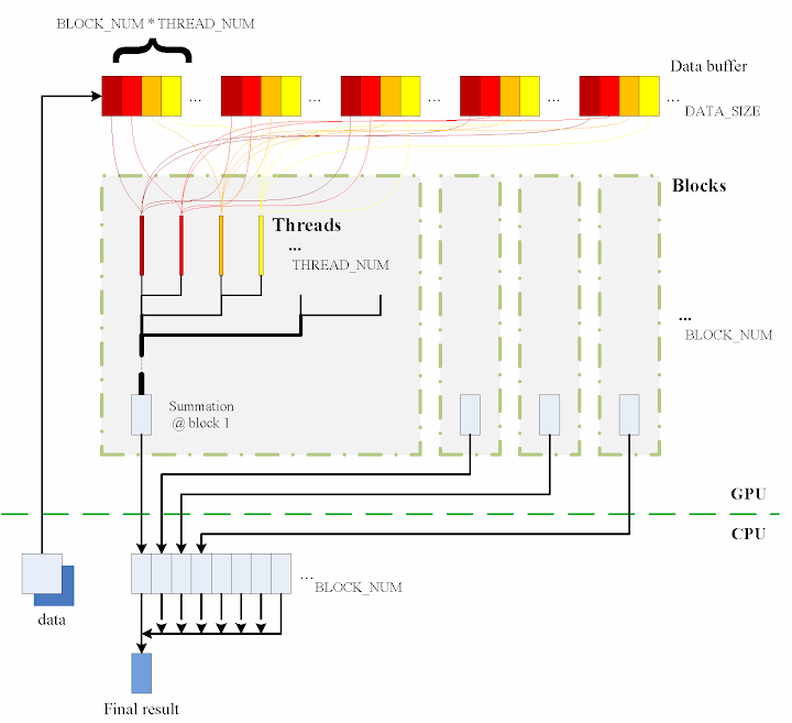
The consecutive steps are:

1. Copy data from the CPU memory to the GPU memory.

cudaMemcpy(gpudata, data, sizeof(int) * DATA_SIZE, cudaMemcpyHostToDevice);

2. Totally BLOCK_NUM blocks are used, and in each block THREAD_NUM threads are produced to perform the calculation. In practice, I used THREAD_NUM = 512, which is the greatest allowed thread number in a block of CUDA. Thereby, the raw data are seperated into DATA_SIZE / (BLOCK_NUM * THREAD_NUM) groups.

3. The access to the data buffer is designed as consecutive, otherwise the efficiency will be reduced.

4. Each thread does its corresponding calculation.

shared[tid] = 0;
for (int i = bid * THREAD_NUM + tid; i < DATA_SIZE; i += BLOCK_NUM * THREAD_NUM) {
    shared[tid] += num[i] * num[i];
}

5. By using shared memory in the blocks, sub summation can be done in each block. Also, the sub summation is parallelised to achieve as high execution speed as possible. Please refer to the source code regarding the details of this part.

6. The BLOCK_NUM sub summation results for all the blocks are copied back to the CPU side, and they are then added together to obtain the final value

cudaMemcpy(&sum, result, sizeof(int) * BLOCK_NUM, cudaMemcpyDeviceToHost);

int final_sum = 0;
for (int i = 0; i < BLOCK_NUM; i++) {
    final_sum += sum[i];
}

Regarding the procedure, function QueryPerformanceCounter records the code execution duration, which is then used for comparison between the different implementations. Before each call of QueryPerformanceCounter, CUDA function cudaThreadSynchronize() is called to make sure that all computations on the GPU are really finished. (Please refer to the CUDA Best Practices Guide §2.1.)

Algorithm in thrust

The application of the library thrust could make the CUDA code as simple as a plain C++ one. The usage of the library is also compatible with the usage of STL (Standard Template Library) of C++. For instance, the code for the calculation on GPU utilising thrust support is scratched like this:

thrust::host_vector<int> data(DATA_SIZE);
srand(time(NULL));
thrust::generate(data.begin(), data.end(), random());

cudaThreadSynchronize();
QueryPerformanceCounter(&elapsed_time_start);

thrust::device_vector<int> gpudata = data;

int final_sum = thrust::transform_reduce(gpudata.begin(), gpudata.end(),
    square<int>(), 0, thrust::plus<int>());

cudaThreadSynchronize();
QueryPerformanceCounter(&elapsed_time_end);
elapsed_time = (double)(elapsed_time_end.QuadPart - elapsed_time_start.QuadPart)
    / frequency.QuadPart;

printf("sum (on GPU): %d; time: %lf\n", final_sum, elapsed_time);

thrust::generate is used to generate the random data, for which the functor random is defined in advance. random was customised to generate a random integer ranged from 0 to 9.

// define functor for
// random number ranged in [0, 9]
class random
{
public:
    int operator() ()
    {
        return rand() % 10;
    }
};

In comparison with the random number generation without thrust, the code could however not be as elegant.

// generate random number ranged in [0, 9]
void GenerateNumbers(int * number, int size)
{
    srand(time(NULL));
    for (int i = 0; i < size; i++) {
        number[i] = rand() % 10;
    }
}

Similarly square is a transformation functor taking one argument. Please refer to the source code for its definition. square was defined for __host__ __device__ and thus it can be used for both the CPU and the GPU sides.

// define transformation f(x) -> x^2
template <typename T>
struct square
{
    __host__ __device__
        T operator() (T x)
    {
        return x * x;
    }
};

That is all for the thrust based code. Is it concise enough? :) Here function QueryPerformanceCounter also records the code duration. On the other hand, the host_vector data is operated on CPU to compare. Using the code below, the summation is performed by the CPU end:

QueryPerformanceCounter(&elapsed_time_start);

final_sum = thrust::transform_reduce(data.begin(), data.end(),
    square<int>(), 0, thrust::plus<int>());

QueryPerformanceCounter(&elapsed_time_end);
elapsed_time = (double)(elapsed_time_end.QuadPart - elapsed_time_start.QuadPart)
    / frequency.QuadPart;

printf("sum (on CPU): %d; time: %lf\n", final_sum, elapsed_time);

I also tested the performance if use thrust::host_vector<int> data as a plain array. This is supposed to cost more overhead, I thought, but we might be curious to know how much. The corresponding code is listed as

final_sum = 0;
for (int i = 0; i < DATA_SIZE; i++)
{
    final_sum += data[i] * data[i];
}

printf("sum (on CPU): %d; time: %lf\n", final_sum, elapsed_time);

The execution time was recorded to compare as well.

Test results on GPU & CPU

The previous experiences show that GPU surpasses CPU when massive parallel computation is realised. When DATA_SIZE increases, the potential of GPU calculation will be gradually released. This is predictable. Moreover, do we lose efficiency when we apply thrust? I guess so, since there is extra cost brought, but do we lose much? We have to judge from the comparison results.
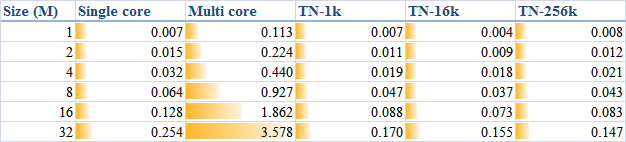
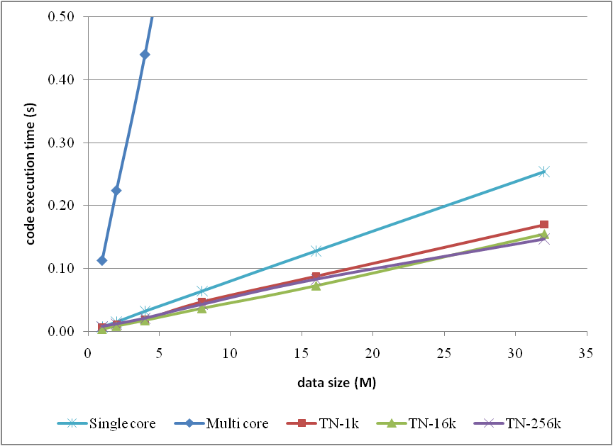
When DATA_SIZE increases from 1 M to 32 M (1 M equals to 1 * 1024 * 1024), the results obtained are illustrated as the table


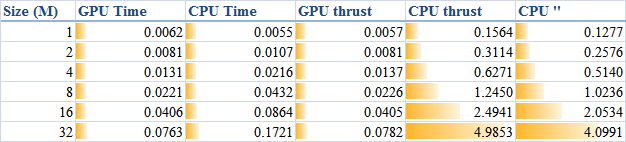
The descriptions of the items are:
  • GPU Time: execution time of the raw CUDA code;
  • CPU Time: execution time of the plain loop code running on the CPU;
  • GPU thrust: execution time of the CUDA code with thrust;
  • CPU thrust: execution time of the CPU code with thrust;
  • CPU '': execution time of the plain loop code based on thrust::
    host_vector
    .
The corresponding trends can be summarised as


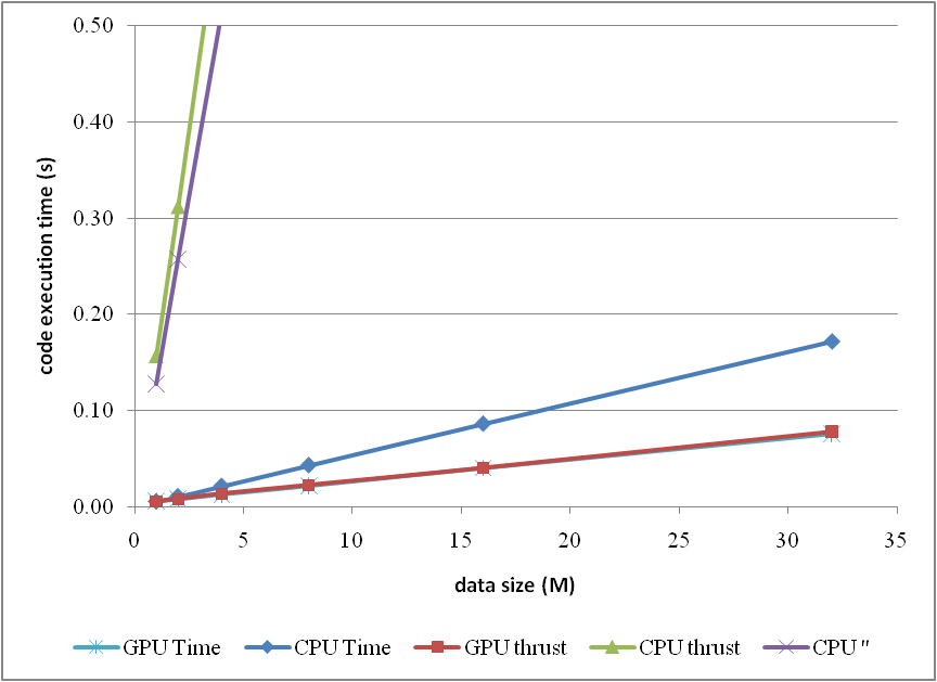
or compare them by the column figure


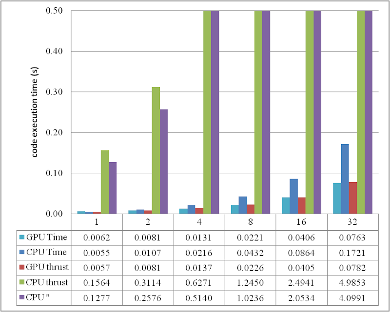
The speedup of GPU to CPU is obvious when DATA_SIZE is more than 4 M. Actually with greater data size, much better performance speedup can be obtained. Interestingly, in this region, the cost of using thrust is quite small, which can even be neglected. However, on the other hand, don't use thrust on the CPU side, neither thrust::transform_reduce method nor a plain loop on a thrust::host_vector; according to the figures, the cost brought is huge. Use a plain array and a loop instead.

From the comparison figure, we found that the application of thrust not only simplifies the code of CUDA computation, but also compensates the loss of efficiency when DATA_SIZE is relatively small. Therefore, it is strongly recommended.

Conclusion

Based on the tests performed, apparently, by employing parallelism, GPU shows greater potential than CPU does, especially for those calculations which contains much more parallel elements. This article also found that the application of thrust does not reduce the code execution efficiency on the GPU side, but brings dramatical negtive changes in the efficiency on the CPU side. Consequently, it is better using plain arrays for CPU calculations.

In conclusion, the usage of thrust feels pretty good, because it improves the code efficiency, and with employing thrust, the CUDA code can be so concise and rapidly developed.

ps - This post can also be referred from one of my articles published on CodeProject, "A brief test on the code efficiency of CUDA and thrust", which could be more complete and source code is attached as well. Any comments are sincerely welcome.

Additionally, the code was built and tested in Windows 7 32 bit plus Visual Studio 2008, CUDA 3.0 and the latest thrust 1.2. One also needs a NVIDIA graphic card as well as CUDA toolkit to run the programs. For instructions on installing CUDA, please refer to its official site CUDA Zone.

Sunday 2 May 2010

Installation of SALOME 5.1.3 on Ubuntu 10.04 (64 bit)

NEW - According to your feedback in the comment list and my own experience, the present tutorial works with SALOME 5.1.5 on Ubuntu 10.10, Kubuntu 10.10 and the latest Ubuntu 11.04.

NEW - As the feedback from vaina, the present tutorial also works with the latest SALOME 5.1.4 on Ubuntu 10.04.

On 23 April 2010, I received the SALOME Newsletter and surprisingly read that they are advising my blog "Free your CFD" for my introduction on SALOME on different platforms. I feel pretty glad and deeply honored because this is definitely the first time I obtain acknowledgement from the SALOME official after my effort during the past more than one years. The part below is from the newsletter.

salome logo Welcome to the April 2010 SALOME Newsletter
...

Solvers' corner

...

"Free your CFD"

Have you bookmarked this blog. It provides useful information and tutorials on Code_Saturne and SALOME.
...
Salome platform logo

To thank you for your support and to celebrate the recent release of the latest Ubuntu 10.04 LTS, I summarise the two previous posts "Installation of SALOME 5.1.1 on Ubuntu 9.04" and "Installation of SALOME 5.1.2 on (K)Ubuntu 9.10 64 bit", test the installation procedure of SALOME version 5.1.3 on Ubuntu 10.04 (64 bit), hereby share my experience and hope it truly helps.

1. Preparation. Although a "Universal binaries for Linux" was released, I still suggest to use the install wizard version to install SALOME, because both of the source code and the corresponding pre-compiled binaries of the necessities are all shipped with the package, and thus it is even possible to share these libraries with Code_Saturne (see "Compile Code_Saturne with SALOME binary libraries").

Install the g++ compiler as SWIG has to be built from source.

:/$ sudo apt-get install build-essential

Replace the executable "sh" with "bash" to avoid some trivial errors.

:/$ sudo rm /bin/sh
:/$ sudo ln -s /bin/bash /bin/sh

Additionally, if it is for a 64 bit Linux, because the install wizard was written for 32 bit, a package ia32-libs is also necessary. It is of course not needed if the Linux environment is 32 bit version.

:/$ sudo apt-get install ia32-libs

Otherwise an error could be encounterred on the console when trying to launch the install wizard.

sh: ./bin/SALOME_InstallWizard: No such file or directory

2. Install. Download the install wizard package and extract it. Ship into the extracted directory and then execute runInstall.

:/$ ./runInstall

Sequentially, the wizard contained 8 steps, for which the screenshots below illustrate. Step 7 is for install progress. After it is started, during the install procedure, there will a warning dialog, shown below as well, poped out, complaining two compulsory libraries, libg2c and libgfortran, haven't been found. Click "OK", ignore the warning and procede until finish the last step of the wizard.


3. Post-install. SALOME has been installed into the $HOME directory; run salome_appli_5.1.3/runAppli to launch the software. However, before the first launch, remember to create a directory USERS under the salome_appli_5.1.3 to avoid an error.

:/$ mkdir salome_appli_5.1.3/USERS
:/$ salome_appli_5.1.3/runAppli &

Up to now, launch SALOME and try to enable the MESH module, an error, shown below, is seen. This is because libg2c and libgfortran are still missing in the system.


To add libgfortran, sequentially execute (note that for Ubuntu 11.04, the libgfortran is in /usr/lib/x86_64-linux-gnu instead of /usr/lib)

:/$ sudo apt-get install gfortran
:/$ sudo ln -s /usr/lib/libgfortran.so.3 /usr/lib/libgfortran.so.1
:/$ sudo ldconfig
:/$ sudo updatedb

To add libg2c, download the packages libg2c0 and gcc-3.4-base (the latter actually provides a dependency for the former one) which suit the system, i386 or amd64, and then install both by dpkg command. For instance, on my Ubuntu 64 bit, execute

:/$ sudo dpkg -i gcc-3.4-base_3.4.6-8ubuntu2_amd64.deb libg2c0_3.4.6-8ubuntu2_amd64.deb

Finally SALOME is supposed to work well.

Monday 22 March 2010

Gambit example: model a 2D channel

"CFD example: laminar flow along a 2D channel" applied SALOME to model and mesh a 2D channel geometry for Code_Saturne to perform the simulation. However, someone likes to use Gambit, a product from ANSYS Fluent, and of course, the same example can also be made with the help of Gambit. Furthermore, similar to SALOME using Python for automatisation, Gambit has Journal file to automatise the manual procedure. The present post aims to translate the previous example into Gambit Journal file in order to show an illustration for beginners.

Basic instructions

1. comments. A comment line in Gambit Journal is headed with a forward slash, /.

/ This line is commented.

2. variables. One is able to define a variable with a name beginning with $. The variable represents a float point value.

$length = 0.1

3. arrays. Array names are also begun with $. In Gambit Journal, array is indexed by a 1 based number, which is quoted by a pair of square parenthesis, []. The index range of an array should be given at the definition declaration of the array itself.

declare $points[1 : 3]
$points[1] = 1.0
$points[2] = 0.0
$points[3] = 0.0

4. For the construction method of points, edges and faces, it is quite concise as well. Please refer to the simple example given in the next section.

The example

Once again, according to the philosophy of executing commands on terminals, Gambit Journal scripts are used to illustrate the example.

///////////////////////////////////////////////////////////////////////
/ Geometry construction and meshing creation for a typical
/ 2d channel flow between two infinite parallel plates.
/
/ Written by: salad
/ Manchester, UK
/ 06/12/2009
///////////////////////////////////////////////////////////////////////
/
/ L = 0.1 m, D = 0.005 m
/
/     C  --------- B
/       |         |
/ -->   |         |
/     O  --------- A
/
/ V_in = 0.05 m/s
/ t    = 50 degree C
///////////////////////////////////////////////////////////////////////

Define the variables and points, and then construct edges and faces accordingly.

/ Variable Definition
$length = 0.1
$height = 0.005

/ points
vertex create "O" coordinates 0
vertex create "A" coordinates $length
vertex create "B" coordinates $length $height
vertex create "C" coordinates 0 $height

/ edges
edge create "OA" straight "O" "A"
edge create "AB" straight "A" "B"
edge create "BC" straight "B" "C"
edge create "CO" straight "C" "O"

/ faces
face create "DUCT" wireframe "OA" "AB" "BC" "CO"

After the geometry is constructed, build the mesh, define the boundaries, and then create a zone corresponding to the 2D face "DUCT". Note that, differing from the SALOME example, here the 2D model is not extruded along the z axis, because originally, I wrote the script for Fluent to use at that moment.

/ mesh
edge mesh "CO" intervals 50
edge mesh "OA" intervals 250
face mesh "DUCT"

/ boundary
physics create "inlet" btype "VELOCITY_INLET" edge "CO"
physics create "bottom" btype "WALL" edge "OA"
physics create "top" btype "WALL" edge "BC"
physics create "outlet" btype "PRESSURE_OUTLET" edge "AB"

/ zones
physics create "duct_v" ctype "FLUID" face "DUCT"

Finally, export the mesh file for future use.

/ export
export uns "2d_duct_flow.msh"

Friday 12 March 2010

MEI is easy to use and works like a charm!

The most expected feature coming from Code_Saturne 2.0-rc1 is the better supported MEI functions. With help of the small CFD calculation case, I tested the feature and have to say that MEI is truly easy to use and works like a charm. Before when I used COMSOL I defined the fluid properties by writting simple MATLAB expressions; (COMSOL is easy to be integrated into MATLAB because originally it is a third party toolbox for MATLAB). It is as easy as you can imagine, and now, within Code_Saturne we are also able to have the same fun.

I used two methods to define the fluid density and viscosity expressions: FORTRAN user routines and MEI expressions. By comparing the results, both methods actually have the same effect. Because I already talked about the first method in the previous tutorial post, I focus on the second one here. Before following, make sure you read "Installation of Code_Saturne 2.0-rc1 on Ubuntu 9.10" and installed 2.0-rc1 with MEI properly.

With the SaturneGUI program, when using 'Physical properties > Fluid properties' to define fluid properties, we have options 'constant', 'user law' and 'user subroutine(usphyv)'. If the property is a constant, fill a value below as a reference value. If select 'user law', MEI expressions can be inputted by clicking the following edit button. Finally, as mentioned previously, the option 'user subroutine' is for using FORTRAN routines to define the properties.


Click the edit button, and see a dialog as the figure below shows. I input a simple density expression as an illustration. Actually there are three tabpages here and the third one also contains an example. TempC is a pre-defined variable, which can be looked up from the second tabpage 'Predefined symbols'. Most operators like +, -, *, /, and ^ can be used, and even simple statements like if ... else can be applied.


Then we don't need to define the temperture dependent density in FORTRAN user routines any more. Obviously this MEI method is more straightforward. I don't say more about the viscosity part, because it is almost the same.

Re-use density value when calculating dynamic viscosity

Dynamic viscosity is the product of density and kinematic viscosity . Sometimes when only a kinematic viscosity expression is available, we need to calculate the dynamic viscosity value with the help of the correlation, .

When using FORTRAN user routines of Code_Saturne, it is possible to realise the correlation directly, which actually implies the previously calculated density value could be read for the viscosity calculating part to use. However, on the other hand, within MEI we don't have a pre-defined symbol, for example rho, to express density when defining a dynamic viscosity mu, and thus we have to expand the rho expression with its original and complicated form into the mu definition expression.

Fortunately, Alexandre gives a patch to implement the idea (see the conversation). After apply the patch accordingly, re-compile ncs, a pre-defined variable rho can then be used for the mu definition. I tested the patch and it works properly.

Post-processing with ParaView

In order to judge whether both methods yield the same effect, the calculation results are analysed. If select to export results into 'EnSight Gold' format, ParaView is going to be used.

ParaView is a cross-platform tool to perform post-processing of numerical simulations. For a beginner I guess it slightly confusing about the mouse controls to move its camera view; at least for me it was true. Actually, select the menu item 'Edit > Settings...' and in the 'Options' dialog ship into the category 'Render View > Camera', can find and modify the controls.


It is not difficult to use ParaView to see the surface plot of a specific parameter, for example, temperature. Select the cell data TempC from the toolbar and the view can then be like this:


From the picture we can see the development of the thermal boundary layer attched to the top and the bottom surfaces of the channel. From the legend the temperature range is found to be 50 to 91.7293 degree C (50 degree C is the inlet temperature), which actually implies the density and viscosity ranges. With MATLAB I estimated them.

>> TempC = [50, 91.7293];
>> rho = 895 ./ (1 + 6.5e-4 .* (TempC - 20))

rho =

  877.8813  855.1304

>> visc = rho .* (0.75857 * (1.8 .* TempC + 32).^-2.34)

visc =

    0.0087    0.0028

Select the data Density and LamVisc in ParaView and see their ranges are 855.12872 to 877.88129 and 0.0027963 to 0.0087367, respectively. They match the results given by MATLAB very well expect the density at 91.7293 degree C, for which there is a very small error, 0.0002%. Thereby, we are happy to see Code_Saturne correctly used the parameter expressions as we expected.

Meanwhile, I compared the results from MEI and FORTRAN user routines, and found their results match exactly, which could imply they have the same effect.

Velocity development along the centreline

Using the filter 'Plot Over Line' we can examine the fluid flow velocity along the centreline of the 2D channel.


Apparently, the velocity rises rapidly at the beginning stage of the channel flow, and then gradually falls. The rise stage is actually within the entrance distance for the flow to be fully developed. On the other hand, the gradual reduction is because of the temperature dependency of the fluid viscosity, as discussed in the previous post "CFD tutorial: laminar flow along a 2D channel - Part I".

Friday 5 March 2010

Installation of Code_Saturne 2.0-rc1 on Ubuntu 9.10

NEW - A post "Installation of Code_Saturne 2.0-rc1 on Ubuntu 10.04 (64 bit)" was recently published and recommended if you have already updated to Ubuntu 10.04.

NEW - On the Code_Saturne forum, David Monfort made very good and useful comments on this post. Please don't miss them.

Code_Saturne 2.0-rc1 is recently released (see the announce, from which all the source packages can be downloaded), and thanks to David's helpful comments on my previous post "Installation of Code_Saturne 2.0.0 on Ubuntu 9.04", I quickly reviewed the installation procedure of this new release, 2.0-rc1. Probably, there can be some interesting points to share with you.

1. Regarding using apt-get to install HDF5 and MED libraries

As advised by David, I found it is easy to install HDF5 and MED by apt-get. libhdf5-dev is a virtual package provided by either one from these:
libhdf5-serial-dev
libhdf5-openmpi-dev
libhdf5-mpich-dev
libhdf5-lam-dev

I explicitly selected libhdf5-openmpi-dev to install. Additionally, hdf5-tools is also necessary to provide h5dump if want to manually compile MED.

$ sudo apt-get install libhdf5-openmpi-dev hdf5-tools

Regarding MED, libmedc-dev is the right one, which depends on another two packages: libmedc1 and libhdf5-serial-1.6.6-0.

sudo apt-get install libmedc-dev

apt-get actually installs slightly older versions of HDF5 and MED, 1.6.6 and 2.3.1, respectively. This is a drawback. More severely, when I 'configure' fvm and ecs, they complained about the old version.
MED >= 2.3.4 headers not found
compatible MED headers not found

Then I think I have to compile MED 2.3.6 by myself.

When trying to compile MED 2.3.6 with the apt-get installed HDF5, I passed the configure but blocked at the make stage.
libtool: compile: gcc -DHAVE_CONFIG_H -I. -I../../include -I../../include -DH5_USE_16_API -g -O2 -MT MEDchampCr.lo -MD -MP -MF .deps/MEDchampCr.Tpo -c MEDchampCr.c -fPIC -DPIC -o .libs/MEDchampCr.o
In file included from /usr/include/hdf5.h:24,
                 from ../../include/med.h:21,
                 from MEDchampCr.c:19:
/usr/include/H5public.h:54:20: error: mpi.h: No such file or directory
/usr/include/H5public.h:56:21: error: mpio.h: No such file or directory

I don't know why but I did install openmpi packages. Ok, since the old version got problems, I turned to compile them again.

2. Process to install 2.0-rc1

If compile the source code, I gladly found most part of the post "Installation of Code_Saturne 2.0.0 on Ubuntu 9.04" can also work well for 2.0-rc1, except the following points:

a. Metis got a confliction with '/usr/include/bits/mathcalls.h'. I am not familiar with this mathcalls.h, but I did a patch to avoid the confliction.
:~/saturne/metis-4.0$ make
(cd Lib ; make )
make[1]: Entering directory `~/saturne/metis-4.0/Lib'
cc -O2 -I. -c coarsen.c
In file included from ./metis.h:36,
                 from coarsen.c:13:
./proto.h:462: error: conflicting types for ‘__log2’
/usr/include/bits/mathcalls.h:145: note: previous declaration of ‘__log2’ was here
make[1]: *** [coarsen.o] Error 1
make[1]: Leaving directory `/home/salad/saturne/metis-4.0/Lib'
make: *** [default] Error 2

We can actually change the function name 'log2' to 'ilog2' in the related head files and source codes under the directory, Lib. The files include: proto.h, rename.h, kmetis.c, kvmetis.c, mkmetis.c and util.c.

You can download my patched version of Metis-4.0 from this link.

b. MEI is now compulsory to be prepared for the compilation of ncs.

It is not difficult to prepare MEI. Firstly, make sure all necessary packages are installed.
:/$ sudo apt-get install bison flex swig python-dev

Then the compilation is easy.

# ship into mei-1.0.1
:/$ ./configure --with-bft=/usr/local
:/$ make
:/$ sudo make install

Note that explicitly specifying --with-bft=/usr/local is necessary for Python to find bft.

c. Regarding ncs, remember to extract the patch file patches-portability-ncs-20rc1.tgz to the ncs directory. When 'configure' ncs, the option 'LIBS=-lm' can be ignored now. It was a bug existing in version 2.0.0-beta2.

# ship into ncs-2.0.0-rc1
:/$ ./configure --with-mpi=/usr/lib/openmpi --with-prepro=/usr/local --with-mei=/usr/local

Once again, an explicit --with-mei=/usr/local is necessary for the python modules.

d. Because there is no eps figure contained in the latex document directories any more, mentioned by David, package texlive-extra-utils is not necessary to install either. However, transfig is still necessary to provide the tool, fig2dev.

# for LaTeX documents
:/$ sudo apt-get install tetex-bin tetex-base transfig

To be honest tetex is already obsoleted from Ubuntu; texlive is much better and can be used instead. I get used to tetex, so I am still using it.

For those who don't use latex elsewhere, maybe installing these huge latex packages to compile Code_Saturne documents seems to be a waste. Don't worry. I prepare my compiled documents (pdf files) here for you to use directly. You can copy the pdf files into the directory /usr/local/share/doc/ncs to let Code_Saturne find them.

e. Before we use command 'cs config' to check the newly installed Code_Saturne status, and then in 2.0-rc1 version, the script 'cs' changes its name to 'code_saturne'.

:/$ code_saturne config

Probably one has to re-create his study and case configurations again with 2.0-rc1, because I tried to open an old xml file, which was previously produced by 2.0.0-beta2, with the SaturneGUI, and it complained that it seems to be for an old version.

3. Future work

The future work ideas are from the mentioned comments, and they include:

a. Different ATLAS packages are provided on Ubuntu for different CPU instruction sets, libatlas-base-dev, libatlas-3dnow-dev, libatlas-sse-dev and libatlas-sse2-dev etc. libatlas-base-dev is only a generic one and should work on every supported CPU architecture. Benchmark could be made to find a most optimised ATLAS package for a specific CPU.

b. MEI is expected to be a very useful feature. With help of MEI, some work, for which FORTRAN user routines have to be written in the past days, can be done by simply expressed formulae. Definitely it is interesting for me to try this.

c. CFDSTUDY is a plugin that allows Code_Saturne to be embedded in the Salome platform. Please read this. An integrated CFD environment can be imagined from this.

d. Last but not least, I tried to apt-get install code-saturne because I know Code_Saturne is already in Debian "unstable" depository. I guess making Code_Saturne available from apt-get might be an ultimate solution for people to install it easily.

salad@salad-desktop:~$ sudo apt-get install code-saturne
Reading package lists... Done
Building dependency tree
Reading state information... Done
Package code-saturne is not available, but is referred to by another package.
This may mean that the package is missing, has been obsoleted, or is only available from another source
E: Package code-saturne has no installation candidate

This actually implies we have to work harder to make an easier life.

Monday 15 February 2010

Post-processing using SALOME and MED

MED file format supports storage of both mesh and simulation results data. SALOME can export its mesh into MED format, and also read result files which are in MED format to perform post-processing operations. Fortunately, Code_Saturne can use MED as its post-processing format. I borrow the figure from a previous post "CFD example: laminar flow along a 2D channel - Part II" to show this. Select the option 'Post-processing format' to 'MED' and then the output result for this case will be in MED.


SALOME's post-processing module can read the Code_Saturne produced MED files, provides many types of operations to show the simulated data, and automatic executive scipt can also be written in Python to control the data presentation styles. The procedure is actually straightforward and it is therefore not the objective of this post. This post aims at revealing another way, which should be more flexible, to access a MED file.

We have compiled MED file library when we try to compile Code_Saturne (please see "Installation of Code_Saturne 2.0.0 on Ubuntu 9.04" for example). The source code of this library is actually shipped with the SALOME installation package (for example, InstallWizard_5.1.3_Debian_4.0_64bit.tar.gz/InstallWizard_5.1.3_Debian_4.0_64bit/Products/SOURCES/med-2.3.6.tar.gz), and the corresponding binary is also included (for example, InstallWizard_5.1.3_Debian_4.0_64bit.tar.gz/InstallWizard_5.1.3_Debian_4.0_64bit/Products/BINARIES/Debian_4.0_64bit/med-2.3.6.tar.gz). Using this library we can write small pieces of code to flexibly access the result data stored in a MED file.

A user guide of MED library can be found from the SALOME install directory DOCUMENTATION_SRC_5.1.3/MEDMEM_UG.pdf. Python scripts to use MED library can be obtained from MED_V5_1_3/bin/salome, for example, the sample file med_test1.py. Following the examples Python code can be written to read a MED file, obtain all the data from it and do whatever operations onto these data, as the flexibility Python provides.

Note that the prepared Python code can only be executed by the Python interpreter shipped with SALOME, which is '$HOME/salome_5.1.3/Python-2.4.4/bin/python'.

It is also possible to write C/C++ code instead of Python if you prefer. For example,

// FIELDuse.cxx
// Written by salad @ Manchester, UK
// 17-08-2009

#include
#include

#include "MEDMEM_Med.hxx"
#include "MEDMEM_Mesh.hxx"
#include "MEDMEM_Field.hxx"

#include "MEDMEM_MedMedDriver.hxx"
#include "MEDMEM_MedMeshDriver.hxx"

using namespace std;
using namespace MEDMEM;

int main(int argc, char ** argv) {
    ...
}

In order to compile the code, firstly, import all the necessary environment variables by executing

:/$ source $HOME/salome_5.1.3/env_products.sh

and Makefile could then be prepared as

# Makefile
# Written by salad @ Manchester, UK
# 17-08-2009

LIB_DIRS = -L${MED_ROOT_DIR}/lib/salome \
    -L${MED2HOME}/lib -L${HDF5HOME}/lib
INCLUDE_DIRS = \
    -I${KERNEL_ROOT_DIR}/include/salome \
    -I${MED_ROOT_DIR}/include/salome \
    -I${MED2HOME}/include -I${HDF5HOME}/include

CFLAGS   = -O -Wno-deprecated -DPCLINUX
MED_LIBS = -lmed -lmedmem -lhdf5 -lz -lgfortran
MODULE   = FIELDuse
SRC      = $(MODULE).cxx
OBJECTS  = $(MODULE).o

all: $(MODULE)

$(OBJECTS): $(SRC)
    g++ -c $(CFLAGS) $(INCLUDE_DIRS) $(SRC)
$(MODULE): $(OBJECTS)
    g++ -o $(MODULE) $(LIB_DIRS) $(OBJECTS) $(MED_LIBS) -pthread

Okay, the last problem is a possibly encountered link error. When linking the code an error says

$HOME/salome_5.1.3/med-2.3.5/lib/libmed.so: undefined reference to `_gfortran_copy_string'

When I was using Ubuntu 9.04 I encountered this problem. I solved it by manually installing gfortran-4.1, which contains the missing functions. Download two packages from "https://launchpad.net/ubuntu/hardy/i386/gcc-4.1-base/4.1.2-21ubuntu1" and "https://launchpad.net/ubuntu/intrepid/i386/libgfortran1/4.1.2-21ubuntu1", and then install them with commands 'sudo dpkg -i'. The error disappeared and a warning left, saying

/usr/bin/ld: warning: libgfortran.so.1, needed by $HOME/salome_5.1.3/med-2.3.5/lib/libmed.so, may conflict with libgfortran.so.3

Ignore it.