I recently ported the CUDA program for 1D heat transfer onto Mac OS X 10.6.8 and CUDA 4.0.31. I only modified the parts related to timing and the program could work perfectly.
The hardware platform comprises GeForce 320M, 950 MHz, and Intel Core 2 Duo P8600, 2.40 GHz. The computation times for GPU and CPU are 1.86 s and 2.15 s respectively; speedup of 1.16. Previously on Windows 7 and CUDA 3.1, GeForce 9800 GTX+ and Q6600 used calculation times 1.43 s and 5.04 s respectively.
The source code is attached for comments.
Showing posts with label Parallel Programming. Show all posts
Showing posts with label Parallel Programming. Show all posts
Sunday, 21 August 2011
Sunday, 26 June 2011
HPCwire interview with NVIDIA's David Kirk
Dr David Kirk is Nvidia's Chief Scientist. Here is an interesting interview with David Kirk on CUDA and parallel computing etc,
GPU Challenges: A Q&A with NVIDIA's David Kirk
GPU Challenges: A Q&A with NVIDIA's David Kirk
Tuesday, 21 September 2010
MATLAB 2010b supports NVIDIA CUDA-capable GPUs
From MATLAB 2010b, GPU support is available in Parallel Computing Toolbox. Using MATLAB for GPU computing lets you take advantage of GPUs without low-level C or Fortran programming.
MATLAB CUDA support provides the base for GPU-accelerated MATLAB operations and lets integrate existing CUDA kernels into MATLAB applications. However, as a restriction, MATLAB only supports GPUs with CUDA compute capability version 1.3 or higher, such as Tesla 10-series and 20-series GPUs. This limitation is not from a light decision; it is actually due to the double precision support and the IEEE-compliant maths implementation of the CUDA capability version 1.3. Please see this thread for more discussion.
MATLAB GPU computing capabilities include:
Introduction to MATLAB GPU Computing (Video)
MATLAB GPU Computing (Documentation)
MATLAB CUDA support provides the base for GPU-accelerated MATLAB operations and lets integrate existing CUDA kernels into MATLAB applications. However, as a restriction, MATLAB only supports GPUs with CUDA compute capability version 1.3 or higher, such as Tesla 10-series and 20-series GPUs. This limitation is not from a light decision; it is actually due to the double precision support and the IEEE-compliant maths implementation of the CUDA capability version 1.3. Please see this thread for more discussion.
MATLAB GPU computing capabilities include:
- Data manipulation on NVIDIA GPUs
- GPU-accelerated MATLAB operations
- Integration of CUDA kernels into MATLAB applications without low-level C or Fortran programming
- Use of multiple GPUs on the desktop (via the toolbox) and a computer cluster (via MATLAB Distributed Computing Server)
Introduction to MATLAB GPU Computing (Video)
MATLAB GPU Computing (Documentation)
Parallel Nsight 1.5 RC with Visual Studio 2010 support
I'm excited to see that the Parallel Nsight 1.5 Release Candidate build (v1.5.10257) is now available at the Parallel Nsight support site. The version introduces compatibility with Visual Studio 2010. You can debug, analyse, and profile your applications in Visual Studio 2010 instead of 2008.
Unfortunately, you will still need the Microsoft v9.0 compilers installed in order to compile your CUDA C/C++ code when using Visual Studio 2010. These compilers ship with Visual Studio 2008, and older versions of the Microsoft Windows SDK.
New Features in Parallel Nsight 1.5 RC:
All:
* Support for Microsoft Visual Studio 2010 in all Parallel Nsight components
* Requires the 260.61 driver (available from the support site)
* Bug fixes and stability improvements
CUDA C/C++ Debugger:
* Support for the CUDA 3.2 RC toolkit
* Support for debugging GPUs using the Tesla Compute Cluster (TCC) driver
* Support for >4GB GPUs, such as the Quadro 6000
* CUDA Memory Checker supports Fermi-based GPUs.
Direct3D Shader Debugger:
* Debugging shaders compiled with the DEBUG flag is now supported.
Direct3D Graphics Inspector:
* Support for GeForce GTX 460 GPUs
* Graphics debug sessions start much faster.
* New Direct3D 11 DXGI texture formats are now supported for visualization.
* Textures used in the current draw call's pixel shader are now viewable directly on the HUD.
Analyzer:
* Support for GeForce GTX 460 GPUs
* NVIDIA Tools Extension (NVTX) events have been improved with color and payload.
* NVIDIA Tools Extension (NVTX) API calls for naming threads, CUDA contexts and other resources
* GPU-side draw call workloads from OpenGL and Direct3D are now traced.
The full release notes can be found at Parallel Nsight support site.
Monday, 2 August 2010
Apply CUDA to solve a 1D heat transfer problem
News - On 27th June, 2010 NVIDIA released CUDA 3.1 and on 21st July, released Parallel Nsight 1.0. The download sites for CUDA Toolkit 3.1 and NVIDIA Parallel Nsight 1.0 are here and here, respectively.
I recently wrote a small piece of code using CUDA to solve a 1D heat transfer problem. The heat transfer happens along the material whose properties are density ρ = 930 kg/m3, specific heat Cp = 1340 J/(kg K) and thermal conductivity k = 0.19 W/(m K). As shown in the figure below, the computation region is illustrated by the thick orange line; the total distance is 1.6 m. There are two boundary conditions attached: at the left end, the temperature is fixed to be 0 oC, while at the right end, a heat flux q = 10 W/m2 is imposed.

If the initial temperature for the entire region is 0 oC, I want to calculate the temperature distribution along the region after 10 seconds' heat propogation.
In the previous figure, the governing heat equation, in partial differential form, has been given. It is then discretised for the internal region, i.e. the orange line, and the right end boundary, which is redly circled, respectively. In the computation, I discretised the entire distance, 1.6 m, into 32768 elements - within CUDA, 64 blocks can be used to handle these elements. On the other hand, for the time marching iteration, the time step can be determined as
^2/4\alpha)
in which α is the thermal diffusivity.
The calculation results, with the help of CUDA and based on float operation, are depicted as

The temperature values for x < 1.5926 m are all zero; therefore they are neglected in the picture. In order to verify the results, the same calculation was also implemented onto CPU and even COMSOL software. The implementation on CPU gave
The interesting thing concerns us is the code efficiency. Once again, I used CUDA 3.1 on my GeForce 9800 GTX+ and a single core of the Q6600 CPU, and the time durations elapsed on the GPU and the CPU for the same calculation are 1.43 s and 5.04 s, respectively. The speedup is 3.52. This speedup value is not that attractive, but it is actually supposed to be much higher when there are much more discretised elements.
I also record the temperature development, in a transient process, of the right end boundary, at which there is heat flux injected. The 10 seconds development curve is illustrated as

I didn't find an easy way to paste source code onto the blog. If you are interested, please leave a comment and the related code can be shared in any way.
I recently wrote a small piece of code using CUDA to solve a 1D heat transfer problem. The heat transfer happens along the material whose properties are density ρ = 930 kg/m3, specific heat Cp = 1340 J/(kg K) and thermal conductivity k = 0.19 W/(m K). As shown in the figure below, the computation region is illustrated by the thick orange line; the total distance is 1.6 m. There are two boundary conditions attached: at the left end, the temperature is fixed to be 0 oC, while at the right end, a heat flux q = 10 W/m2 is imposed.
If the initial temperature for the entire region is 0 oC, I want to calculate the temperature distribution along the region after 10 seconds' heat propogation.
In the previous figure, the governing heat equation, in partial differential form, has been given. It is then discretised for the internal region, i.e. the orange line, and the right end boundary, which is redly circled, respectively. In the computation, I discretised the entire distance, 1.6 m, into 32768 elements - within CUDA, 64 blocks can be used to handle these elements. On the other hand, for the time marching iteration, the time step can be determined as
in which α is the thermal diffusivity.
The calculation results, with the help of CUDA and based on float operation, are depicted as
The temperature values for x < 1.5926 m are all zero; therefore they are neglected in the picture. In order to verify the results, the same calculation was also implemented onto CPU and even COMSOL software. The implementation on CPU gave
The interesting thing concerns us is the code efficiency. Once again, I used CUDA 3.1 on my GeForce 9800 GTX+ and a single core of the Q6600 CPU, and the time durations elapsed on the GPU and the CPU for the same calculation are 1.43 s and 5.04 s, respectively. The speedup is 3.52. This speedup value is not that attractive, but it is actually supposed to be much higher when there are much more discretised elements.
I also record the temperature development, in a transient process, of the right end boundary, at which there is heat flux injected. The 10 seconds development curve is illustrated as
I didn't find an easy way to paste source code onto the blog. If you are interested, please leave a comment and the related code can be shared in any way.
News - The source code can be found in the new post on porting this CUDA program onto Mac OS X.
Sunday, 11 July 2010
A brief test on the efficiency of a .NET 4.0 parallel code example - Part II
With respect to the article, "A Brief Test on the Efficiency of a .NET 4.0 Parallel Code Example", Daniel Grunwald proposed additional interesting pieces of code to compare. First of all, the LINQ and PLINQ methods are present as
They are the most concise code to implement the computation. However, when the individual calculations are very cheap, for example, this simple multiplication d => d * d, the overhead of delegates and lambda expressions could be largely noticable.
When parallelising an algorithm, it is essential to avoid false sharing. In the previous article I split the raw data array into a group of pieces and compute the sub-summation for each piece. Actually I manually determine the number of the pieces - I did a sensitivity study and found that 16 k pieces are sufficient for a data size less than 32 M; larger data size might need more pieces.
Daniel reminded that, by using an advanced overload of Parallel.For, the work can be distributed into pieces by .NET. The code is as
However this method didn't improve the efficiency as expected, at least not efficient as my manual method grouping the array into 16 k pieces, because of, we believe, the dramatic overhead caused by delegates relatively to the cheap multiply-add operation.
Then the working units can be combined to be slightly heavier to compensate the delegate overhead, for example, processing 1024 elements in each invocation.
Finally, this piece of code becomes the most efficient one we have ever found.
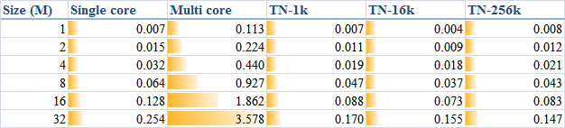
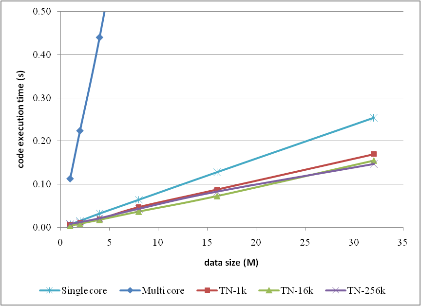
In order to generally look at the comparison between the methods, I, once again, list a table as

and the corresponding curves

Note that, in the comparison, I neglected the methods which have already been proved as inefficient in the previous article for clarity.
Any comments are welcome.
// LINQ (running on single core)

final_sum = data.Sum(d => d * d);

// PLINQ (parallelised)

final_sum = data.AsParallel().Sum(d => d * d);
They are the most concise code to implement the computation. However, when the individual calculations are very cheap, for example, this simple multiplication d => d * d, the overhead of delegates and lambda expressions could be largely noticable.
When parallelising an algorithm, it is essential to avoid false sharing. In the previous article I split the raw data array into a group of pieces and compute the sub-summation for each piece. Actually I manually determine the number of the pieces - I did a sensitivity study and found that 16 k pieces are sufficient for a data size less than 32 M; larger data size might need more pieces.
Daniel reminded that, by using an advanced overload of Parallel.For, the work can be distributed into pieces by .NET. The code is as
// localSum

final_sum = 0;

Parallel.For(0, DATA_SIZE,

             () => 0, // initialization for each thread

             (i, s, localSum) => localSum + data[i] * data[i], // loop body

             localSum => Interlocked.Add(ref final_sum, localSum) // final action for each thread

            );
However this method didn't improve the efficiency as expected, at least not efficient as my manual method grouping the array into 16 k pieces, because of, we believe, the dramatic overhead caused by delegates relatively to the cheap multiply-add operation.
Then the working units can be combined to be slightly heavier to compensate the delegate overhead, for example, processing 1024 elements in each invocation.
// localSum & groups

final_sum = 0;

Parallel.For(0, (int)(DATA_SIZE / 1024),

             () => 0,

             (i, s, localSum) =>

             {

                 int end = (i + 1) * 1024;

                 for (int j = i * 1024; j < end; j++)

                 {

                     localSum += data[j] * data[j];

                 }

                 return localSum;

             },

             localSum => Interlocked.Add(ref final_sum, localSum)

            );
Finally, this piece of code becomes the most efficient one we have ever found.
In order to generally look at the comparison between the methods, I, once again, list a table as
and the corresponding curves
Note that, in the comparison, I neglected the methods which have already been proved as inefficient in the previous article for clarity.
Any comments are welcome.
Friday, 2 July 2010
A brief test on the efficiency of a .NET 4.0 parallel code example
As a piece of accompanying work of the article, "A short test on the code efficiency of CUDA and thrust", I published a new parallel code example in C# 4.0 on CodeProject. The new example tests the new parallel programming support provided from .NET 4.0, and the corresponding article can be found as
A Brief Test on the Efficiency of a .NET 4.0 Parallel Code Example
Briefly the test results could be depicted by
and pictorially
however the original text is suggested to read for more details if you are interested.
I hope the work helps and your comments are welcome.
A Brief Test on the Efficiency of a .NET 4.0 Parallel Code Example
Briefly the test results could be depicted by
and pictorially
however the original text is suggested to read for more details if you are interested.
I hope the work helps and your comments are welcome.
Saturday, 22 May 2010
A short test on the code efficiency of CUDA and thrust
Introduction
Numerical simulations are always pretty time consuming jobs. Most of these jobs take lots of hours to complete, even though multi-core CPUs are commonly used. Before I can afford a cluster, how to dramatically improve the calculation efficiency on my desktop computers to save computational effort became a critical problem I am facing and dreaming to achieve.
NVIDIA CUDA seems more and more popular and potential to solve the present problem with the power released from GPU. CUDA framework provides a modified C language and with its help my C programming experiences can be re-used to implement numerical algorithms by utilising a GPU. Whilst thrust is a C++ template library for CUDA. thrust is aimed at improving developers' development productivity; however, the code execution efficiency is also of high priority for a numerical job. Someone stated that code execution efficiency could be lost to some extent due to the extra cost from using the library thrust. To judge this precisely, I did a series of basic tests in order to explore the truth. Basically, that is the purpose of this article.
My personal computer is a Intel Q6600 quad core CPU plus 3G DDR2 800M memory. Although I don't have good hard drives, marked only 5.1 in Windows 7 32 bit, I think in this test of the calculation of the summation of squares, the access to hard drives might not be significant. The graphic card used is a GeForce 9800 GTX+ with 512M GDDR3 memory. The card is shown as

Algorithm in raw CUDA
The test case I used is solving the summation of squares of an array of integers (random numbers ranged from 0 to 9), and, as I mentioned, a GeForce 9800 GTX+ graphic card running within Windows 7 32-bit system was employed for the testing. If in plain C language, the summation could be implemented by the following loop code, which is then executed on a CPU core:
Obviously, it is a serial computation. The code is executed in a serial stream of instructions. In order to utilise the power of CUDA, the algorithm has to be parallelised, and the more parallelisation are realised, the more potential power will be explored. With the help of my basic understanding on CUDA, I split the data into different groups and then used the equivalent number of threads on the GPU to calculate the summation of the squares of each group. Ultimately results from all the groups are added together to obtain the final result.
The algorithm designed is briefly shown in the figure
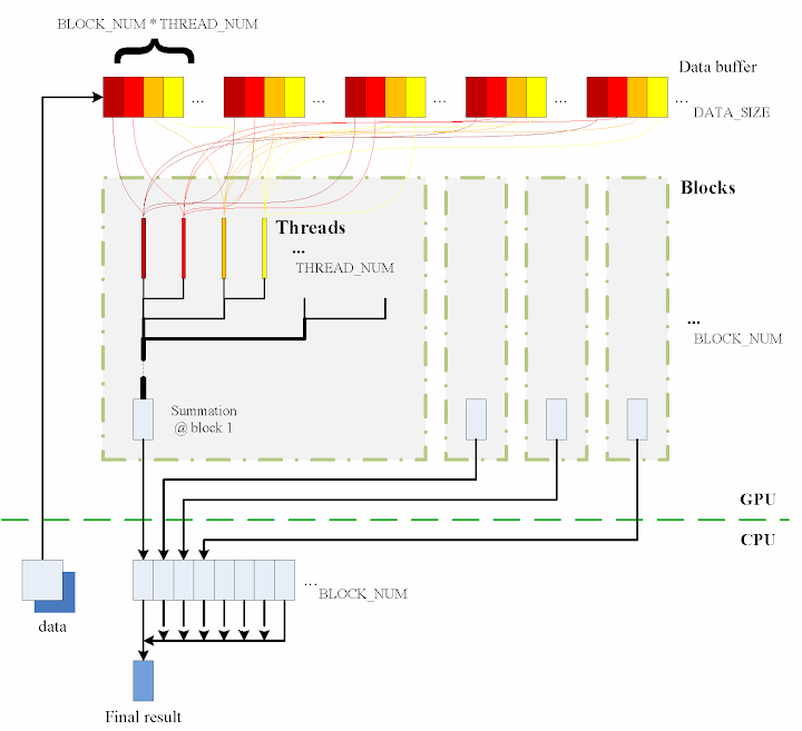
The consecutive steps are:
1. Copy data from the CPU memory to the GPU memory.
2. Totally BLOCK_NUM blocks are used, and in each block THREAD_NUM threads are produced to perform the calculation. In practice, I used THREAD_NUM = 512, which is the greatest allowed thread number in a block of CUDA. Thereby, the raw data are seperated into DATA_SIZE / (BLOCK_NUM * THREAD_NUM) groups.
3. The access to the data buffer is designed as consecutive, otherwise the efficiency will be reduced.
4. Each thread does its corresponding calculation.
5. By using shared memory in the blocks, sub summation can be done in each block. Also, the sub summation is parallelised to achieve as high execution speed as possible. Please refer to the source code regarding the details of this part.
6. The BLOCK_NUM sub summation results for all the blocks are copied back to the CPU side, and they are then added together to obtain the final value
Regarding the procedure, function QueryPerformanceCounter records the code execution duration, which is then used for comparison between the different implementations. Before each call of QueryPerformanceCounter, CUDA function cudaThreadSynchronize() is called to make sure that all computations on the GPU are really finished. (Please refer to the CUDA Best Practices Guide §2.1.)
Algorithm in thrust
The application of the library thrust could make the CUDA code as simple as a plain C++ one. The usage of the library is also compatible with the usage of STL (Standard Template Library) of C++. For instance, the code for the calculation on GPU utilising thrust support is scratched like this:
thrust::generate is used to generate the random data, for which the functor random is defined in advance. random was customised to generate a random integer ranged from 0 to 9.
In comparison with the random number generation without thrust, the code could however not be as elegant.
Similarly square is a transformation functor taking one argument. Please refer to the source code for its definition. square was defined for __host__ __device__ and thus it can be used for both the CPU and the GPU sides.
That is all for the thrust based code. Is it concise enough? :) Here function QueryPerformanceCounter also records the code duration. On the other hand, the host_vector data is operated on CPU to compare. Using the code below, the summation is performed by the CPU end:
I also tested the performance if use thrust::host_vector<int> data as a plain array. This is supposed to cost more overhead, I thought, but we might be curious to know how much. The corresponding code is listed as
The execution time was recorded to compare as well.
Test results on GPU & CPU
The previous experiences show that GPU surpasses CPU when massive parallel computation is realised. When DATA_SIZE increases, the potential of GPU calculation will be gradually released. This is predictable. Moreover, do we lose efficiency when we apply thrust? I guess so, since there is extra cost brought, but do we lose much? We have to judge from the comparison results.
When DATA_SIZE increases from 1 M to 32 M (1 M equals to 1 * 1024 * 1024), the results obtained are illustrated as the table
The descriptions of the items are:
or compare them by the column figure
The speedup of GPU to CPU is obvious when DATA_SIZE is more than 4 M. Actually with greater data size, much better performance speedup can be obtained. Interestingly, in this region, the cost of using thrust is quite small, which can even be neglected. However, on the other hand, don't use thrust on the CPU side, neither thrust::transform_reduce method nor a plain loop on a thrust::host_vector; according to the figures, the cost brought is huge. Use a plain array and a loop instead.
From the comparison figure, we found that the application of thrust not only simplifies the code of CUDA computation, but also compensates the loss of efficiency when DATA_SIZE is relatively small. Therefore, it is strongly recommended.
Conclusion
Based on the tests performed, apparently, by employing parallelism, GPU shows greater potential than CPU does, especially for those calculations which contains much more parallel elements. This article also found that the application of thrust does not reduce the code execution efficiency on the GPU side, but brings dramatical negtive changes in the efficiency on the CPU side. Consequently, it is better using plain arrays for CPU calculations.
In conclusion, the usage of thrust feels pretty good, because it improves the code efficiency, and with employing thrust, the CUDA code can be so concise and rapidly developed.
Numerical simulations are always pretty time consuming jobs. Most of these jobs take lots of hours to complete, even though multi-core CPUs are commonly used. Before I can afford a cluster, how to dramatically improve the calculation efficiency on my desktop computers to save computational effort became a critical problem I am facing and dreaming to achieve.
NVIDIA CUDA seems more and more popular and potential to solve the present problem with the power released from GPU. CUDA framework provides a modified C language and with its help my C programming experiences can be re-used to implement numerical algorithms by utilising a GPU. Whilst thrust is a C++ template library for CUDA. thrust is aimed at improving developers' development productivity; however, the code execution efficiency is also of high priority for a numerical job. Someone stated that code execution efficiency could be lost to some extent due to the extra cost from using the library thrust. To judge this precisely, I did a series of basic tests in order to explore the truth. Basically, that is the purpose of this article.
My personal computer is a Intel Q6600 quad core CPU plus 3G DDR2 800M memory. Although I don't have good hard drives, marked only 5.1 in Windows 7 32 bit, I think in this test of the calculation of the summation of squares, the access to hard drives might not be significant. The graphic card used is a GeForce 9800 GTX+ with 512M GDDR3 memory. The card is shown as
Algorithm in raw CUDA
The test case I used is solving the summation of squares of an array of integers (random numbers ranged from 0 to 9), and, as I mentioned, a GeForce 9800 GTX+ graphic card running within Windows 7 32-bit system was employed for the testing. If in plain C language, the summation could be implemented by the following loop code, which is then executed on a CPU core:
int final_sum = 0;

for (int i = 0; i < DATA_SIZE; i++) {

    final_sum += data[i] * data[i];

}
Obviously, it is a serial computation. The code is executed in a serial stream of instructions. In order to utilise the power of CUDA, the algorithm has to be parallelised, and the more parallelisation are realised, the more potential power will be explored. With the help of my basic understanding on CUDA, I split the data into different groups and then used the equivalent number of threads on the GPU to calculate the summation of the squares of each group. Ultimately results from all the groups are added together to obtain the final result.
The algorithm designed is briefly shown in the figure
The consecutive steps are:
1. Copy data from the CPU memory to the GPU memory.
cudaMemcpy(gpudata, data, sizeof(int) * DATA_SIZE, cudaMemcpyHostToDevice);
2. Totally BLOCK_NUM blocks are used, and in each block THREAD_NUM threads are produced to perform the calculation. In practice, I used THREAD_NUM = 512, which is the greatest allowed thread number in a block of CUDA. Thereby, the raw data are seperated into DATA_SIZE / (BLOCK_NUM * THREAD_NUM) groups.
3. The access to the data buffer is designed as consecutive, otherwise the efficiency will be reduced.
4. Each thread does its corresponding calculation.
shared[tid] = 0;

for (int i = bid * THREAD_NUM + tid; i < DATA_SIZE; i += BLOCK_NUM * THREAD_NUM) {

    shared[tid] += num[i] * num[i];

}
5. By using shared memory in the blocks, sub summation can be done in each block. Also, the sub summation is parallelised to achieve as high execution speed as possible. Please refer to the source code regarding the details of this part.
6. The BLOCK_NUM sub summation results for all the blocks are copied back to the CPU side, and they are then added together to obtain the final value
cudaMemcpy(&sum, result, sizeof(int) * BLOCK_NUM, cudaMemcpyDeviceToHost);


int final_sum = 0;

for (int i = 0; i < BLOCK_NUM; i++) {

    final_sum += sum[i];

}
Regarding the procedure, function QueryPerformanceCounter records the code execution duration, which is then used for comparison between the different implementations. Before each call of QueryPerformanceCounter, CUDA function cudaThreadSynchronize() is called to make sure that all computations on the GPU are really finished. (Please refer to the CUDA Best Practices Guide §2.1.)
Algorithm in thrust
The application of the library thrust could make the CUDA code as simple as a plain C++ one. The usage of the library is also compatible with the usage of STL (Standard Template Library) of C++. For instance, the code for the calculation on GPU utilising thrust support is scratched like this:
thrust::host_vector<int> data(DATA_SIZE);

srand(time(NULL));

thrust::generate(data.begin(), data.end(), random());


cudaThreadSynchronize();

QueryPerformanceCounter(&elapsed_time_start);


thrust::device_vector<int> gpudata = data;


int final_sum = thrust::transform_reduce(gpudata.begin(), gpudata.end(),

    square<int>(), 0, thrust::plus<int>());


cudaThreadSynchronize();

QueryPerformanceCounter(&elapsed_time_end);

elapsed_time = (double)(elapsed_time_end.QuadPart - elapsed_time_start.QuadPart)

    / frequency.QuadPart;


printf("sum (on GPU): %d; time: %lf\n", final_sum, elapsed_time);
thrust::generate is used to generate the random data, for which the functor random is defined in advance. random was customised to generate a random integer ranged from 0 to 9.
// define functor for

// random number ranged in [0, 9]

class random

{

public:

    int operator() ()

    {

        return rand() % 10;

    }

};
In comparison with the random number generation without thrust, the code could however not be as elegant.
// generate random number ranged in [0, 9]

void GenerateNumbers(int * number, int size)

{

    srand(time(NULL));

    for (int i = 0; i < size; i++) {

        number[i] = rand() % 10;

    }

}
Similarly square is a transformation functor taking one argument. Please refer to the source code for its definition. square was defined for __host__ __device__ and thus it can be used for both the CPU and the GPU sides.
// define transformation f(x) -> x^2

template <typename T>

struct square

{

    __host__ __device__

        T operator() (T x)

    {

        return x * x;

    }

};
That is all for the thrust based code. Is it concise enough? :) Here function QueryPerformanceCounter also records the code duration. On the other hand, the host_vector data is operated on CPU to compare. Using the code below, the summation is performed by the CPU end:
QueryPerformanceCounter(&elapsed_time_start);


final_sum = thrust::transform_reduce(data.begin(), data.end(),

    square<int>(), 0, thrust::plus<int>());


QueryPerformanceCounter(&elapsed_time_end);

elapsed_time = (double)(elapsed_time_end.QuadPart - elapsed_time_start.QuadPart)

    / frequency.QuadPart;


printf("sum (on CPU): %d; time: %lf\n", final_sum, elapsed_time);
I also tested the performance if use thrust::host_vector<int> data as a plain array. This is supposed to cost more overhead, I thought, but we might be curious to know how much. The corresponding code is listed as
final_sum = 0;

for (int i = 0; i < DATA_SIZE; i++)

{

    final_sum += data[i] * data[i];

}


printf("sum (on CPU): %d; time: %lf\n", final_sum, elapsed_time);
The execution time was recorded to compare as well.
Test results on GPU & CPU
The previous experiences show that GPU surpasses CPU when massive parallel computation is realised. When DATA_SIZE increases, the potential of GPU calculation will be gradually released. This is predictable. Moreover, do we lose efficiency when we apply thrust? I guess so, since there is extra cost brought, but do we lose much? We have to judge from the comparison results.
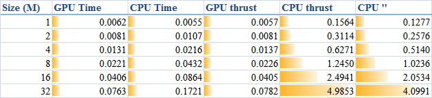
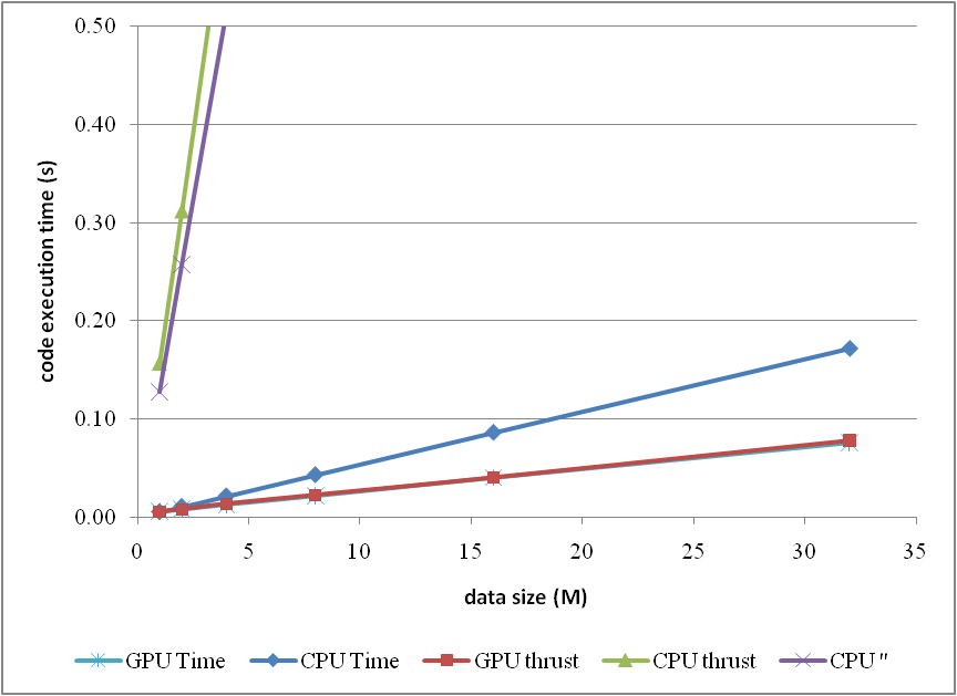
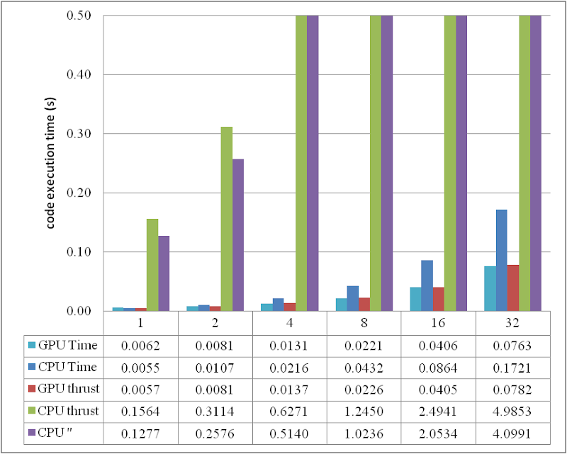
When DATA_SIZE increases from 1 M to 32 M (1 M equals to 1 * 1024 * 1024), the results obtained are illustrated as the table
The descriptions of the items are:
- GPU Time: execution time of the raw CUDA code;
- CPU Time: execution time of the plain loop code running on the CPU;
- GPU thrust: execution time of the CUDA code with thrust;
- CPU thrust: execution time of the CPU code with thrust;
- CPU '': execution time of the plain loop code based on thrust::
host_vector.
or compare them by the column figure
The speedup of GPU to CPU is obvious when DATA_SIZE is more than 4 M. Actually with greater data size, much better performance speedup can be obtained. Interestingly, in this region, the cost of using thrust is quite small, which can even be neglected. However, on the other hand, don't use thrust on the CPU side, neither thrust::transform_reduce method nor a plain loop on a thrust::host_vector; according to the figures, the cost brought is huge. Use a plain array and a loop instead.
From the comparison figure, we found that the application of thrust not only simplifies the code of CUDA computation, but also compensates the loss of efficiency when DATA_SIZE is relatively small. Therefore, it is strongly recommended.
Conclusion
Based on the tests performed, apparently, by employing parallelism, GPU shows greater potential than CPU does, especially for those calculations which contains much more parallel elements. This article also found that the application of thrust does not reduce the code execution efficiency on the GPU side, but brings dramatical negtive changes in the efficiency on the CPU side. Consequently, it is better using plain arrays for CPU calculations.
In conclusion, the usage of thrust feels pretty good, because it improves the code efficiency, and with employing thrust, the CUDA code can be so concise and rapidly developed.
ps - This post can also be referred from one of my articles published on CodeProject, "A brief test on the code efficiency of CUDA and thrust", which could be more complete and source code is attached as well. Any comments are sincerely welcome.
Additionally, the code was built and tested in Windows 7 32 bit plus Visual Studio 2008, CUDA 3.0 and the latest thrust 1.2. One also needs a NVIDIA graphic card as well as CUDA toolkit to run the programs. For instructions on installing CUDA, please refer to its official site CUDA Zone.
Additionally, the code was built and tested in Windows 7 32 bit plus Visual Studio 2008, CUDA 3.0 and the latest thrust 1.2. One also needs a NVIDIA graphic card as well as CUDA toolkit to run the programs. For instructions on installing CUDA, please refer to its official site CUDA Zone.
Subscribe to:
Posts (Atom)


