Monday 15 February 2010

Post-processing using SALOME and MED

MED file format supports storage of both mesh and simulation results data. SALOME can export its mesh into MED format, and also read result files which are in MED format to perform post-processing operations. Fortunately, Code_Saturne can use MED as its post-processing format. I borrow the figure from a previous post "CFD example: laminar flow along a 2D channel - Part II" to show this. Select the option 'Post-processing format' to 'MED' and then the output result for this case will be in MED.


SALOME's post-processing module can read the Code_Saturne produced MED files, provides many types of operations to show the simulated data, and automatic executive scipt can also be written in Python to control the data presentation styles. The procedure is actually straightforward and it is therefore not the objective of this post. This post aims at revealing another way, which should be more flexible, to access a MED file.

We have compiled MED file library when we try to compile Code_Saturne (please see "Installation of Code_Saturne 2.0.0 on Ubuntu 9.04" for example). The source code of this library is actually shipped with the SALOME installation package (for example, InstallWizard_5.1.3_Debian_4.0_64bit.tar.gz/InstallWizard_5.1.3_Debian_4.0_64bit/Products/SOURCES/med-2.3.6.tar.gz), and the corresponding binary is also included (for example, InstallWizard_5.1.3_Debian_4.0_64bit.tar.gz/InstallWizard_5.1.3_Debian_4.0_64bit/Products/BINARIES/Debian_4.0_64bit/med-2.3.6.tar.gz). Using this library we can write small pieces of code to flexibly access the result data stored in a MED file.

A user guide of MED library can be found from the SALOME install directory DOCUMENTATION_SRC_5.1.3/MEDMEM_UG.pdf. Python scripts to use MED library can be obtained from MED_V5_1_3/bin/salome, for example, the sample file med_test1.py. Following the examples Python code can be written to read a MED file, obtain all the data from it and do whatever operations onto these data, as the flexibility Python provides.

Note that the prepared Python code can only be executed by the Python interpreter shipped with SALOME, which is '$HOME/salome_5.1.3/Python-2.4.4/bin/python'.

It is also possible to write C/C++ code instead of Python if you prefer. For example,

// FIELDuse.cxx
// Written by salad @ Manchester, UK
// 17-08-2009

#include
#include

#include "MEDMEM_Med.hxx"
#include "MEDMEM_Mesh.hxx"
#include "MEDMEM_Field.hxx"

#include "MEDMEM_MedMedDriver.hxx"
#include "MEDMEM_MedMeshDriver.hxx"

using namespace std;
using namespace MEDMEM;

int main(int argc, char ** argv) {
    ...
}

In order to compile the code, firstly, import all the necessary environment variables by executing

:/$ source $HOME/salome_5.1.3/env_products.sh

and Makefile could then be prepared as

# Makefile
# Written by salad @ Manchester, UK
# 17-08-2009

LIB_DIRS = -L${MED_ROOT_DIR}/lib/salome \
    -L${MED2HOME}/lib -L${HDF5HOME}/lib
INCLUDE_DIRS = \
    -I${KERNEL_ROOT_DIR}/include/salome \
    -I${MED_ROOT_DIR}/include/salome \
    -I${MED2HOME}/include -I${HDF5HOME}/include

CFLAGS   = -O -Wno-deprecated -DPCLINUX
MED_LIBS = -lmed -lmedmem -lhdf5 -lz -lgfortran
MODULE   = FIELDuse
SRC      = $(MODULE).cxx
OBJECTS  = $(MODULE).o

all: $(MODULE)

$(OBJECTS): $(SRC)
    g++ -c $(CFLAGS) $(INCLUDE_DIRS) $(SRC)
$(MODULE): $(OBJECTS)
    g++ -o $(MODULE) $(LIB_DIRS) $(OBJECTS) $(MED_LIBS) -pthread

Okay, the last problem is a possibly encountered link error. When linking the code an error says

$HOME/salome_5.1.3/med-2.3.5/lib/libmed.so: undefined reference to `_gfortran_copy_string'

When I was using Ubuntu 9.04 I encountered this problem. I solved it by manually installing gfortran-4.1, which contains the missing functions. Download two packages from "https://launchpad.net/ubuntu/hardy/i386/gcc-4.1-base/4.1.2-21ubuntu1" and "https://launchpad.net/ubuntu/intrepid/i386/libgfortran1/4.1.2-21ubuntu1", and then install them with commands 'sudo dpkg -i'. The error disappeared and a warning left, saying

/usr/bin/ld: warning: libgfortran.so.1, needed by $HOME/salome_5.1.3/med-2.3.5/lib/libmed.so, may conflict with libgfortran.so.3

Ignore it.

Saturday 6 February 2010

CFD tutorial: laminar flow along a 2D channel - Part II

Geometry and mesh using SALOME

Please read Part I of this article.

CFD solving with Code_Saturne

After the mesh file is produced from SALOME, Code_Saturne can be used for a CFD calculation. Note that I take Code_Saturne 2.0.0 as an example in this post; if you are still using Code_Saturne 1.x, remember some commands and directory names are different.

1. Create a study with a case.

Command 'cs create' is for this. Use option '--help' to get its help message, '-s' and '-c' to specify a study name and a case name, respectively. Note that from 2.0-rc1 version, the script name cs is changed to code_saturne; please use code_saturne instead if you are using Code_Saturne 2.0-rc1. (Within Code_Saturne 1.x, command 'cree_sat -etude' has to be used instead; for clarity, this post doesn't include the content related to version 1.x.)

:/$ cs create --help
:/$ cs create -s DUCT -c 2D

With the command executed, a study directory named 'DUCT' and a case called '2D' are created. In the directory 'DUCT', there are three sub-directories:

*. 2D: The case directory. A study can have several cases; for example, different boundary conditions can be organised as different cases.
*. MESH: Code_Saturne will read mesh files from this directory, and as such we need to copy mesh files into it;
*. POST: This is an empty directory designed to contain post-processing macros (xmgrace, experimental etc).

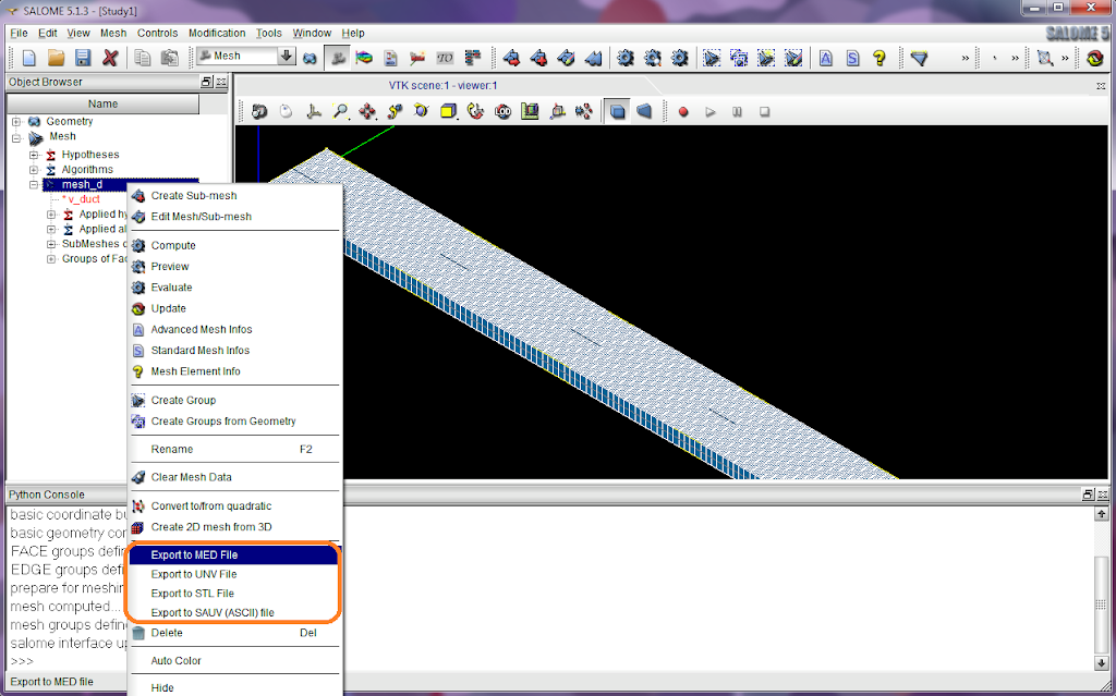
Copy the mesh file 'mesh_d.med' into the directory 'MESH'. Then we look at the case directory '2D', in which there are four sub-directories:

*. DATA: Contains the script to launch the GUI SaturneGUI.
*. RESU: Directory where the results will be exported once the calculation has finished.
*. SCRIPTS: The launching scripts are copied here. The CFD calculation is actually started by executing the launching script 'runcase' here.
*. SRC: The user subroutines are saved here. During the compilation stage, the code will re-compile all the subroutines that are in this directory. In the 'REFERENCE' directory all the user-defined subroutines are stored. For a specific case you will only need a few of them depending on the changes that you want to implement on the code. The 'base' directory contains the basic flow solver subroutines, and the other directories contain the subroutines needed by other modules.

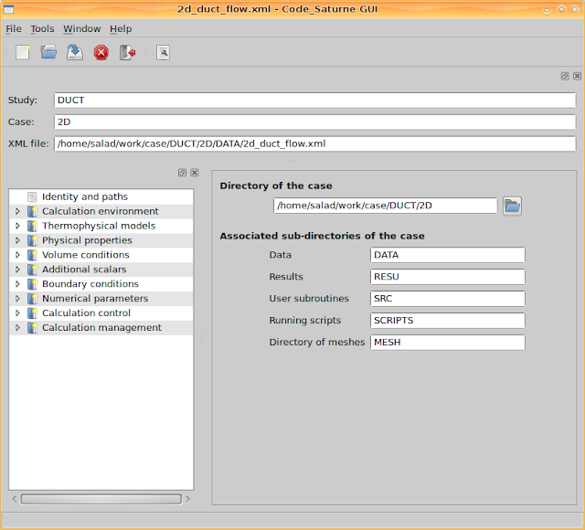
2. Use GUI to input parameters. Ship into the directory 'DUCT/2D/DATA' and then execute 'SaturneGUI' to launch the GUI.

:/$ ./SaturneGUI &

The parameters set with the GUI can actually be saved into a XML file, and as such for a second time to launch the GUI, option '-f' can be used to load the XML file directly.

:/$ ./SaturneGUI -f 2d_duct_flow.xml &

The first glance at the GUI is like this. It lists the structure of directories. With the help of the navigator at the left panel, we can go to different pages to modify various parameters.


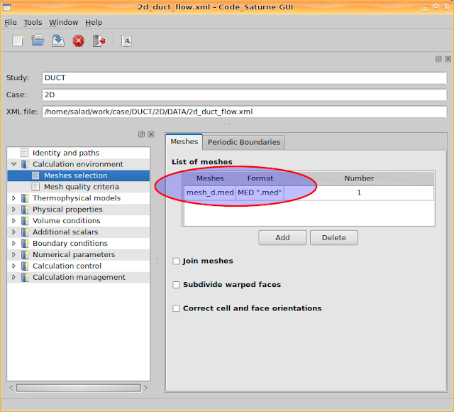
Go to 'Calculation environment > Meshes selection' and add the mesh file 'mesh_d.med'. It can recognise mesh files from the directory 'MESH'.


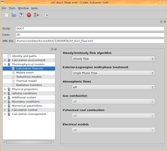
Go to 'Thermophysical models > Calculation features' and enable two features, 'steady flow' and 'single Phase Flow'.


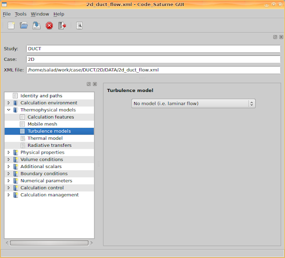
Go to 'Thermophysical models > Turbulence models' and select 'No model (i.e. laminar flow), since we ignore turbulence and only consider a laminar approximation. Besides, select the 'Thermal scalar' to be 'Temperature (Celsius)' on the page 'Thermal model' and select 'No radiative transfers' on the page 'Radiative transfers' as we ignore radiation.


Go to 'Physical properties > Fluid properties' and set the four fluid properties: density, viscosity, specific heat and thermal conductivity. As shown in the following figure, we set specific heat and thermal conductivity as constant values, and leave density and viscosity to the user subroutine 'usphyv'. Therefore, the reference values set for density and viscosity do not matter.

In 'usphyv' the parameters could be controlled as temperature dependent. It will be discussed in the next section.


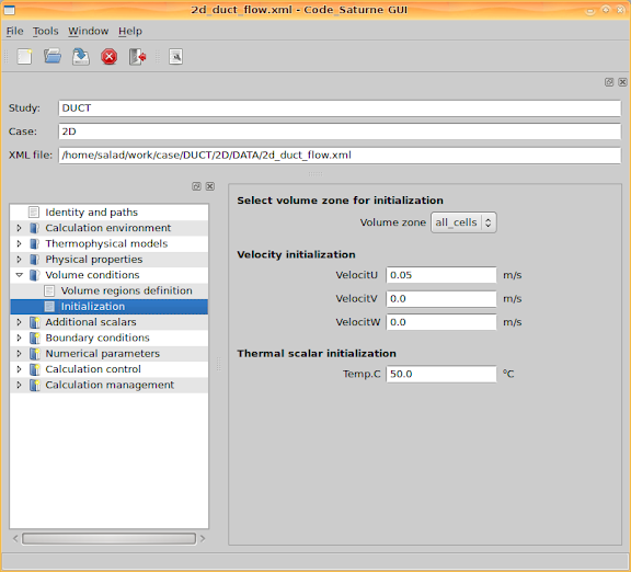
Go to 'Volume conditions > Initialization' and set initial values for velocity and temperature. Here I set the x component of the velocity as the inlet velocity value, and set the temperature as the inlet temperature value.


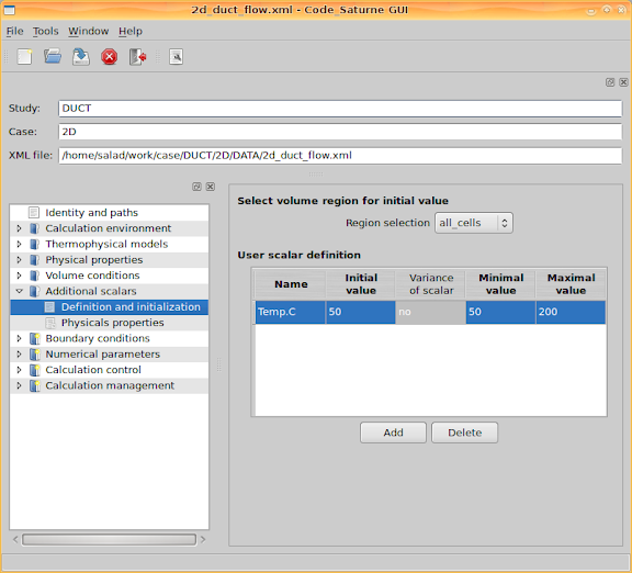
Go to 'Additional scalars > Definition and initialization' and set the scalar limitation for temperature, including its minimal and maximal values.


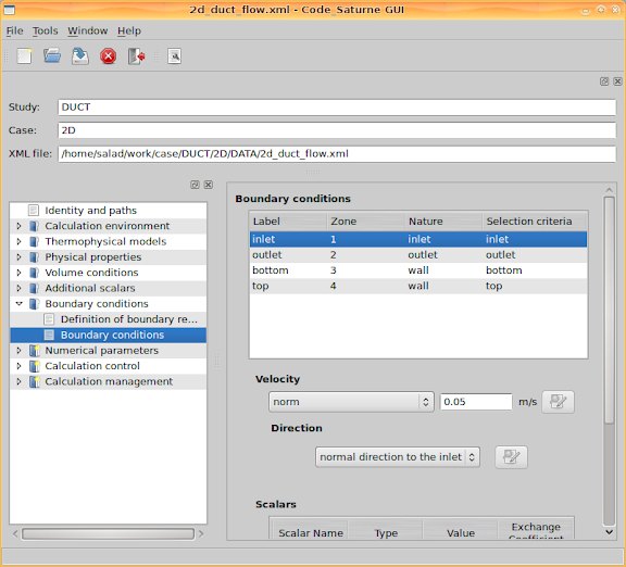
Next step is about boundary conditions. Firstly, boundaries have to be defined. Since we used SALOME to generate the mesh, according to the defined mesh groups, inlet, outlet, bottom, top and sym, corresponding boundaries can be defined. For more details about the mesh groups, please see Part I of this article.


Secondly, go to 'Boundary conditions > Boundary conditions' and set values for the boundaries. I set the inlet velocity and temperature, and set minus heat flux values at the two walls. Negative heat flux means the heat is into the channel. Additionally, the walls are set as smooth walls.


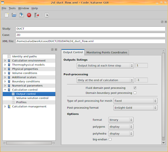
Leave 'Numerical parameters' with the default values, and go to 'Calculation control > Output control'. Then set 'Output listing at each time step', set output 'Post-processing' 'Only at the end of calculation' since we are concerning a steady state calculation result.

With respect to the 'Post-processing format', either 'Ensight Gold' or 'MED' can be specified. If you prefer to use ParaView, select 'Ensight Gold'. If you want to use SALOME to do post-processing, change the option to 'MED'.


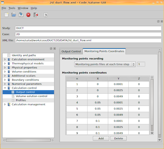
Then go to the second tab page. This page lists the 'Monitoring points coordinates'. When the calculation is being performed, the quantity values at these coordinates will be recorded for each iteration step (each time step if it is a transient process).


Once the calculation is started, we can go to Saturne's temporary directory to check the history data at these monitored points. For example, to check the x component of velocity, use 'xmgrace'

~/tmp_Saturne/DUCT.2D.02061151$ xmgrace -nxy probes_VelocitU.dat

The result could be like this figure below, from which we can see all the values are already stable after 70 iteration steps. It implies a criterion to stop the calculation after a number of steps.
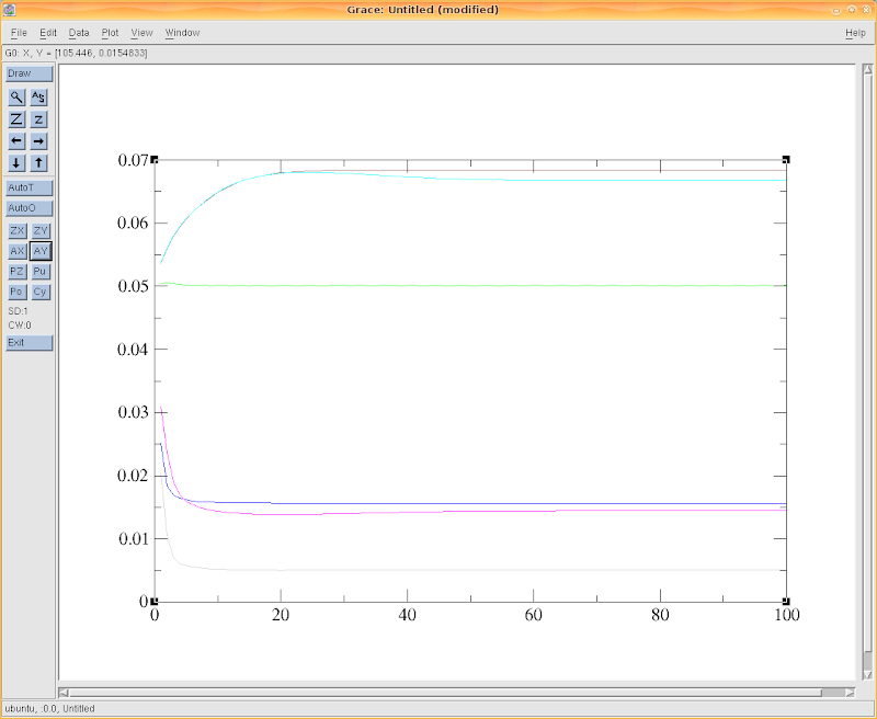

Actually cs plot_probes command instead of xmgrace -nxy could be used to draw the graph of the values at the probes; it's a wrapper around xmgrace with a couple of file manipulation.

3. Apply FORTRAN user routines.

As mentioned the fluid density and viscosity could be configured as temperature dependent by modifying user routines in 'usphyv.f90'. Adopting FORTRAN code to control the calculation details brings enough flexibility to Code_Saturne.

All user routines/FORTRAN files are put in the directory 'SRC'. Look up the sub-directory 'REFERENCE' and see all the routines you can modify. For fluid properties, copy the file SRC/REFERENCE/base/usphyv.f90 into SRC and then modify the copied file in SRC.

For density, search the corresponding piece of code in the file and then modify the part as the following code list, which defines the density expression


T is temperature. Actually 0.00065 is the fluid expansion coefficient due to temperature.

iutile = 1
! ...

! --- Coefficients des lois choisis et imposes par l'utilisateur
!     Les valeurs donnees ici sont fictives

vara = 895
varb = 0.00065
varc = 20

! Masse volumique au centre des cellules
! ---------------------------------------
! loi  RHO = A / (1 + B * (T - C))
! soit PROPCE(IEL,IPCROM) = VARA / (1 + VARB * (XRTP - VARC))

do iel = 1, ncel
  xrtp = rtp(iel, ivart)
  propce(iel, ipcrom) = vara / (1 + varb * (xrtp - varc))
enddo

Note that the first line set the variable 'iutile' to 1, otherwise the code implementing the equation will not take effect.

For viscosity, find the code piece, assign 'iutile' 1 and modify the following code as whatever viscosity equation you would try. With the density code example, it is not supposed to be difficult.

!===============================================================================
!  EXEMPLE 2 : VISCOSITE VARIABLE EN FONCTION DE LA TEMPERATURE
! ===========
! ...

iutile = 1
! ...

4. Solve.

After configured all the necessary aspects and modified the user routines, go to 'Calculation management > Prepare batch calculation' and we are able to start the CFD calculation right now. Firstly, 'Select the batch script file', i.e. click the button to browser a launch script file. As default, the file is named 'runcase'.


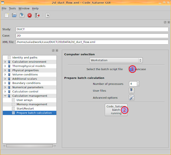
Then select the 'Number of processors', and click the button 'Code_Saturne batch running'. A console window will pop out and Code_Saturne will produce code to do the calculation. I assume that you are using more than one processor cores to calculate, and then you might be asked for your Linux system user password by openmpi before the calculation.

Leave the calculation console for minutes and then, if lucky enough, you will see the calculation finished normally. If so, the next step is to see the results and do post-processing.

Post-processing with ParaView

Please read Part III of this article.

CFD tutorial: laminar flow along a 2D channel - Part I

When fluid flows along a 2D channel, which is between two infinite parallel plates, with a relatively low velocity (laminar flow), a hydraulic stable status can be achieved after a certain distance (entrance length). This stable flow status is named as hydraulically fully developed flow. Furthermore, if there is heat flux at the duct surfaces, the fluid near the wall will be warmed up, and a thermal boundary layer is then formed.

For a flow along a channel without heated, after it is fully developed, the velocity pattern at a cross area is parabolic. However, if the flow is also heated, the parabolic velocity pattern will be twisted because of the viscosity dependency of the fluid (this is true for many types of liquid). This phenomenon is pictorially shown as the figure below, in which (a) is the parabolic velocity profile, and (b) is the distorted profile in a heated duct due to the temperature dependency of the fluid viscosity.


Denote the duct height as H, duct length as L, fluid density as , and the average velocity in the duct region as U. Then the pressure drop between the two ends of the duct can be expressed as


in which is defined as friction coefficient. Actually this equation says the active pressure force has to balance the friction force due to shear stress, which is finally related to the fluid viscosity.

Anyway, I select this example to show a simple CFD calculation, because its simple geometry. Using SALOME we can very quickly build up a geometry and then mesh it. Probably an expected structured mesh of the channel can be like this. It is better to have dense mesh near the inlet and the walls of the duct.


Geometry and mesh using SALOME

According to the philosophy of executing commands on terminals, I'll use python scripts to re-perform the procedure of modelling in SALOME.

#######################################################################
# Geometry construction and meshing creation for a typical
# 2d channel flow between two infinite parallel plates.
#
# Written by: salad
# Manchester, UK
# 06/02/2010
#######################################################################

How to execute these scripts? New a blank study in SALOME and then a 'Python Console' can be seen at the bottom of the window. Input or copy scripts into the console and press Enter to execute them. Scripts can also be saved in a .py file, and with the menu item 'File >> Load Script...' a dialog 'Load python script' can help load script files and execute them as a batch. 'Ctrl+T' is the shortcut to call the dialog.

Ok, let's start. 1. Import the necessary libraries and define the related dimensions. We are going to build a duct with height 5 mm and length 100 mm.

import os
import sys
import salome
from math import *
from geompy import *
import copy

# basic unit
unit = 0.001
# extrusion length
extru = unit

duct_height = unit * 5
duct_length = unit * 100

'extru' is the extrusion length along the z axis. This length will be meshed with only one cell. Actually Code_Saturne only handles 3D meshes with FVM. Therefore, to simulate a 2D mesh, it is a good practice to extrude the 2D mesh with a 1 cell layer thickness.

2. Build the basic coordinate.

#
# basic coordinate
#
p0 = MakeVertex(0, 0, 0)
dx = MakeVectorDXDYDZ(unit, 0, 0)
dy = MakeVectorDXDYDZ(0, unit, 0)
dz = MakeVectorDXDYDZ(0, 0, unit)
addToStudy(p0, "p0")
addToStudy(dx, "dx")
addToStudy(dy, "dy")
addToStudy(dz, "dz")

print "basic coordinate built..."

3. Construct the channel geometry. The geometry modelling procedure can be briefly expressed as: points => edges => faces => extrusion. Points are constructed with coordinates, edges are defined by linking points, and faces are then defined by specifying its edges. Finally extrusion helps convert the 2D geometry to 3D.

#
# geometry construction
#

# points
p1 = MakeVertex(duct_length, 0, 0)
p2 = MakeVertex(0, duct_height, 0)
p3 = MakeVertex(duct_length, duct_height, 0)

# build edges
e0 = MakeEdge(p0, p1)
e1 = MakeEdge(p2, p3)
e2 = MakeEdge(p0, p2)
e3 = MakeEdge(p1, p3)

# build face
f_duct = MakeFaceWires([e0, e1, e2, e3], 1)

# extrude along the z axis
v_duct = MakePrismVecH(f_duct, dz, extru)
addToStudy(v_duct, "v_duct")

print "channel geometry constructed..."

4. Define the groups. Groups are necessary because they correspond to the boundaries used during CFD calculations. Here we define the geometry groups and these groups will then be encapsulated into mesh groups later. Mesh groups will be used to define boundary conditions when using Code_Saturne.

Firstly, define the face groups. Functions used in the python script can be looked up in the SALOME document.

# FACE groups definition:
# 1. inlet
# 2. outlet
# 3. bottom
# 4. top
# 5. sym

# sym is declared and filled
sub_faces = SubShapeAllSorted(v_duct, ShapeType["FACE"])
g_sym = CreateGroup(v_duct, ShapeType["FACE"])
UnionList(g_sym, sub_faces)

# inlet
sub_faces = GetShapesOnPlane(v_duct, ShapeType["FACE"], dx, GEOM.ST_ON)

g_inlet = CreateGroup(v_duct, ShapeType["FACE"])
UnionList(g_inlet, sub_faces)
DifferenceList(g_sym, sub_faces)

addToStudyInFather(v_duct, g_inlet, "inlet")

# outlet
sub_faces = GetShapesOnPlaneWithLocation(v_duct, ShapeType["FACE"], dx, p1, GEOM.ST_ON)

g_outlet = CreateGroup(v_duct, ShapeType["FACE"])
UnionList(g_outlet, sub_faces)
DifferenceList(g_sym, sub_faces)

addToStudyInFather(v_duct, g_outlet, "outlet")

# bottom
sub_faces = GetShapesOnPlane(v_duct, ShapeType["FACE"], dy, GEOM.ST_ON)

g_bottom = CreateGroup(v_duct, ShapeType["FACE"])
UnionList(g_bottom, sub_faces)
DifferenceList(g_sym, sub_faces)

addToStudyInFather(v_duct, g_bottom, "bottom")

# top
sub_faces = GetShapesOnPlaneWithLocation(v_duct, ShapeType["FACE"], dy, p2, GEOM.ST_ON)

g_top = CreateGroup(v_duct, ShapeType["FACE"])
UnionList(g_top, sub_faces)
DifferenceList(g_sym, sub_faces)

addToStudyInFather(v_duct, g_top, "top")

# sym is finally obtained
addToStudyInFather(v_duct, g_sym, "sym")

print "FACE groups defined..."

Then define the edge groups.

# EDGE groups definition:
# 1. let (inlet & outlet of the channel)
# 2. tb (top & bottom of the channel)
# 3. extru (the extrusion length)

# let
g_let = GetEdgesByLength(v_duct, duct_height, duct_height, 1, 1)
addToStudyInFather(v_duct, g_let, "let")

# tb
g_tb = GetEdgesByLength(v_duct, duct_length, duct_length, 1, 1)
addToStudyInFather(v_duct, g_tb, "tb")

# extru
g_extru = GetEdgesByLength(v_duct, extru, extru, 1, 1)
addToStudyInFather(v_duct, g_extru, "extru")

print "EDGE groups defined..."

5. Mesh. Till now the geometry is already produced. Meshing can be performed with the script below. Note that the expressions, which define the corresponding mesh density profiles, can be edited to any others if necessary.

#
# meshing
#
import smesh
import StdMeshers

mesh_d = smesh.Mesh(v_duct, "mesh_d")

print "prepare for meshing..."

# construction of mesh

# as default, a 1D edge is meshed with only 1 cell
# it is for the extrusion length
algo1d = mesh_d.Segment()
algo1d.NumberOfSegments(1)

# structured rectangular mesh is preferred for 2D faces
algo2d = mesh_d.Quadrangle()
algo2d.QuadranglePreference()

algo3d = mesh_d.Hexahedron()

# submesh

# for inlet & outlet, use parabolic mesh density profile
algo1d_let = mesh_d.Segment(g_let)
seg = algo1d_let.NumberOfSegments(50)
seg.SetDistrType(3)
seg.SetConversionMode(1)
seg.SetExpressionFunction('(t-0.5)^2+0.1')

# for top & bottom, use a decreasing profile from the inlet to the outlet
algo1d_tb = mesh_d.Segment(g_tb)
seg = algo1d_tb.NumberOfSegments(250)
seg.SetDistrType(3)
seg.SetConversionMode(0)
seg.SetExpressionFunction('(t-1)^4+0.1')

status = mesh_d.Compute()

print "mesh computed..."

The same with the geometry modelling, groups of mesh are also defined accordingly.

#
# mesh groups
#

mesh_d.GroupOnGeom(g_inlet, "inlet")
mesh_d.GroupOnGeom(g_outlet, "outlet")
mesh_d.GroupOnGeom(g_bottom, "bottom")
mesh_d.GroupOnGeom(g_top, "top")
mesh_d.GroupOnGeom(g_sym, "sym")

print "mesh groups defined..."

Arriving at this, you should be able to update the SALOME GUI to see the mesh generated, and also judge whether it is what you want.

# update
salome.sg.updateObjBrowser(1)

6. Output. After the mesh is produced, it has to be saved into a file before using it with Code_Saturne. In SALOME, right-click the object 'mesh_d' and from the context menu we can see that SALOME supports exporting to MED and UNV file formats. If your Code_Saturne was compiled with MED support, I recommend to use MED because of its smaller file size; or UNV can be used.


Finally a file 'mesh_d.med' (or 'mesh_d.unv') is obtained. This is the mesh file we will move to Code_Saturne's MESH directory.

CFD solving with Code_Saturne

Please read Part II of this article.

Post-processing with ParaView

Please read Part III of this article.