Please read Part I of this article.
CFD solving with Code_Saturne
After the mesh file is produced from SALOME, Code_Saturne can be used for a CFD calculation. Note that I take Code_Saturne 2.0.0 as an example in this post; if you are still using Code_Saturne 1.x, remember some commands and directory names are different.
1. Create a study with a case.
Command 'cs create' is for this. Use option '--help' to get its help message, '-s' and '-c' to specify a study name and a case name, respectively. Note that from 2.0-rc1 version, the script name cs is changed to code_saturne; please use code_saturne instead if you are using Code_Saturne 2.0-rc1. (Within Code_Saturne 1.x, command 'cree_sat -etude' has to be used instead; for clarity, this post doesn't include the content related to version 1.x.)
:/$ cs create --help

:/$ cs create -s DUCT -c 2D
With the command executed, a study directory named 'DUCT' and a case called '2D' are created. In the directory 'DUCT', there are three sub-directories:
*. 2D: The case directory. A study can have several cases; for example, different boundary conditions can be organised as different cases.
*. MESH: Code_Saturne will read mesh files from this directory, and as such we need to copy mesh files into it;
*. POST: This is an empty directory designed to contain post-processing macros (xmgrace, experimental etc).
Copy the mesh file 'mesh_d.med' into the directory 'MESH'. Then we look at the case directory '2D', in which there are four sub-directories:
*. DATA: Contains the script to launch the GUI SaturneGUI.
*. RESU: Directory where the results will be exported once the calculation has finished.
*. SCRIPTS: The launching scripts are copied here. The CFD calculation is actually started by executing the launching script 'runcase' here.
*. SRC: The user subroutines are saved here. During the compilation stage, the code will re-compile all the subroutines that are in this directory. In the 'REFERENCE' directory all the user-defined subroutines are stored. For a specific case you will only need a few of them depending on the changes that you want to implement on the code. The 'base' directory contains the basic flow solver subroutines, and the other directories contain the subroutines needed by other modules.
2. Use GUI to input parameters. Ship into the directory 'DUCT/2D/DATA' and then execute 'SaturneGUI' to launch the GUI.
:/$ ./SaturneGUI &
The parameters set with the GUI can actually be saved into a XML file, and as such for a second time to launch the GUI, option '-f' can be used to load the XML file directly.
:/$ ./SaturneGUI -f 2d_duct_flow.xml &
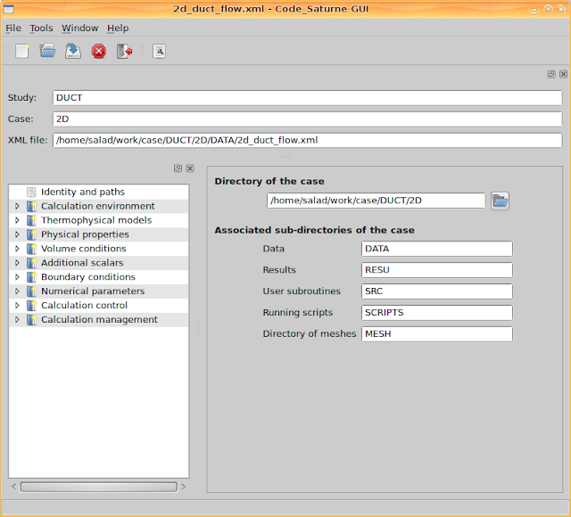
The first glance at the GUI is like this. It lists the structure of directories. With the help of the navigator at the left panel, we can go to different pages to modify various parameters.
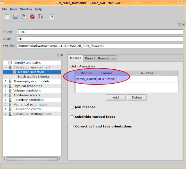
Go to 'Calculation environment > Meshes selection' and add the mesh file 'mesh_d.med'. It can recognise mesh files from the directory 'MESH'.
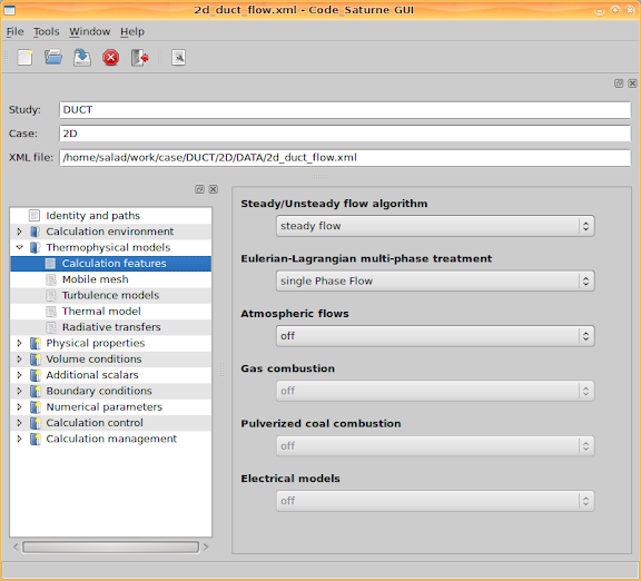
Go to 'Thermophysical models > Calculation features' and enable two features, 'steady flow' and 'single Phase Flow'.
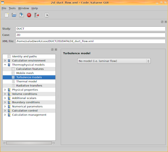
Go to 'Thermophysical models > Turbulence models' and select 'No model (i.e. laminar flow), since we ignore turbulence and only consider a laminar approximation. Besides, select the 'Thermal scalar' to be 'Temperature (Celsius)' on the page 'Thermal model' and select 'No radiative transfers' on the page 'Radiative transfers' as we ignore radiation.
Go to 'Physical properties > Fluid properties' and set the four fluid properties: density, viscosity, specific heat and thermal conductivity. As shown in the following figure, we set specific heat and thermal conductivity as constant values, and leave density and viscosity to the user subroutine 'usphyv'. Therefore, the reference values set for density and viscosity do not matter.
In 'usphyv' the parameters could be controlled as temperature dependent. It will be discussed in the next section.

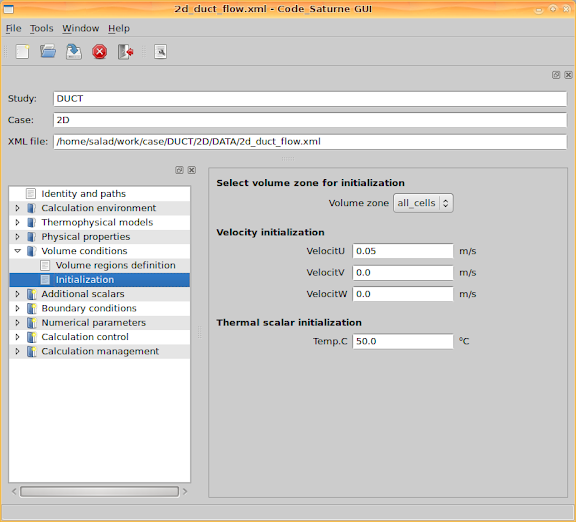
Go to 'Volume conditions > Initialization' and set initial values for velocity and temperature. Here I set the x component of the velocity as the inlet velocity value, and set the temperature as the inlet temperature value.
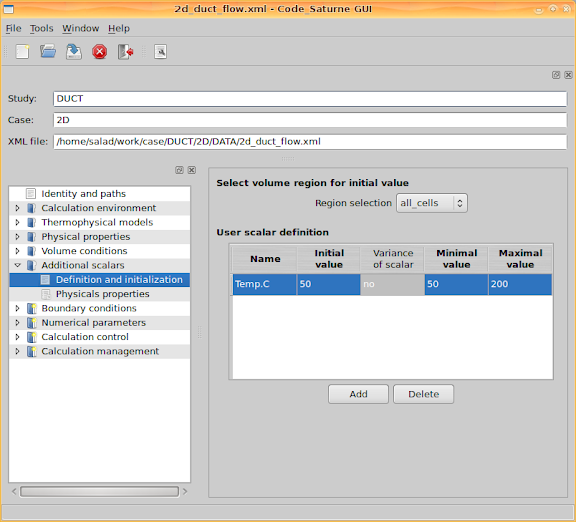
Go to 'Additional scalars > Definition and initialization' and set the scalar limitation for temperature, including its minimal and maximal values.
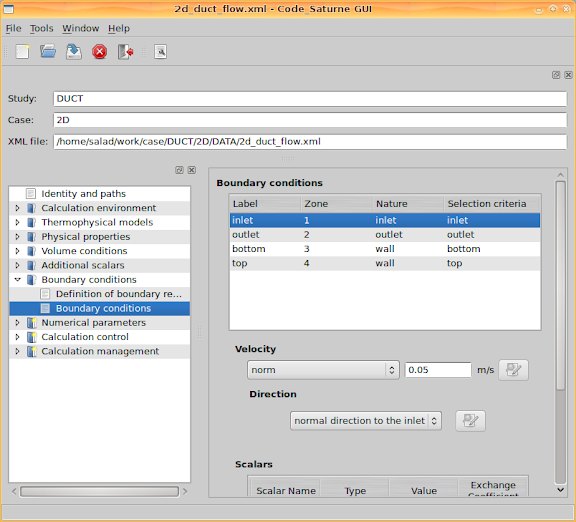
Next step is about boundary conditions. Firstly, boundaries have to be defined. Since we used SALOME to generate the mesh, according to the defined mesh groups, inlet, outlet, bottom, top and sym, corresponding boundaries can be defined. For more details about the mesh groups, please see Part I of this article.

Secondly, go to 'Boundary conditions > Boundary conditions' and set values for the boundaries. I set the inlet velocity and temperature, and set minus heat flux values at the two walls. Negative heat flux means the heat is into the channel. Additionally, the walls are set as smooth walls.
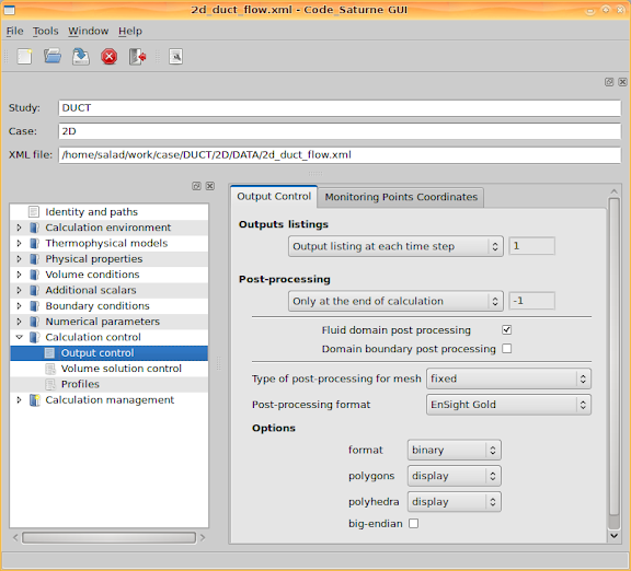
Leave 'Numerical parameters' with the default values, and go to 'Calculation control > Output control'. Then set 'Output listing at each time step', set output 'Post-processing' 'Only at the end of calculation' since we are concerning a steady state calculation result.
With respect to the 'Post-processing format', either 'Ensight Gold' or 'MED' can be specified. If you prefer to use ParaView, select 'Ensight Gold'. If you want to use SALOME to do post-processing, change the option to 'MED'.
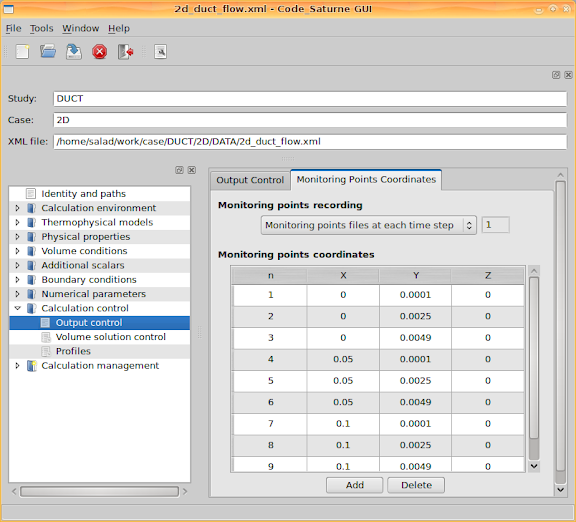
Then go to the second tab page. This page lists the 'Monitoring points coordinates'. When the calculation is being performed, the quantity values at these coordinates will be recorded for each iteration step (each time step if it is a transient process).
Once the calculation is started, we can go to Saturne's temporary directory to check the history data at these monitored points. For example, to check the x component of velocity, use 'xmgrace'
~/tmp_Saturne/DUCT.2D.02061151$ xmgrace -nxy probes_VelocitU.dat
The result could be like this figure below, from which we can see all the values are already stable after 70 iteration steps. It implies a criterion to stop the calculation after a number of steps.
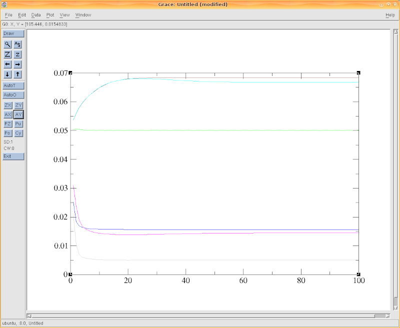_VelocitU.png)
Actually cs plot_probes command instead of xmgrace -nxy could be used to draw the graph of the values at the probes; it's a wrapper around xmgrace with a couple of file manipulation.
3. Apply FORTRAN user routines.
As mentioned the fluid density and viscosity could be configured as temperature dependent by modifying user routines in 'usphyv.f90'. Adopting FORTRAN code to control the calculation details brings enough flexibility to Code_Saturne.
All user routines/FORTRAN files are put in the directory 'SRC'. Look up the sub-directory 'REFERENCE' and see all the routines you can modify. For fluid properties, copy the file SRC/REFERENCE/base/usphyv.f90 into SRC and then modify the copied file in SRC.
For density, search the corresponding piece of code in the file and then modify the part as the following code list, which defines the density expression
T is temperature. Actually 0.00065 is the fluid expansion coefficient due to temperature.
iutile = 1

! ...


! --- Coefficients des lois choisis et imposes par l'utilisateur

!     Les valeurs donnees ici sont fictives


vara  =  895

varb  =  0.00065

varc  =  20


! Masse volumique au centre des cellules

! ---------------------------------------

!     loi  RHO = A / (1 + B * (T - C))

!     soit      PROPCE(IEL,IPCROM) = VARA / (1 + VARB * (XRTP - VARC))


do iel = 1, ncel

  xrtp = rtp(iel, ivart)

  propce(iel, ipcrom) = vara / (1 + varb * (xrtp - varc))

enddo
Note that the first line set the variable 'iutile' to 1, otherwise the code implementing the equation will not take effect.
For viscosity, find the code piece, assign 'iutile' 1 and modify the following code as whatever viscosity equation you would try. With the density code example, it is not supposed to be difficult.
!===============================================================================

!  EXEMPLE 2 : VISCOSITE       VARIABLE EN FONCTION DE LA TEMPERATURE

! ===========

! ...


iutile = 1

! ...
4. Solve.
After configured all the necessary aspects and modified the user routines, go to 'Calculation management > Prepare batch calculation' and we are able to start the CFD calculation right now. Firstly, 'Select the batch script file', i.e. click the button to browser a launch script file. As default, the file is named 'runcase'.
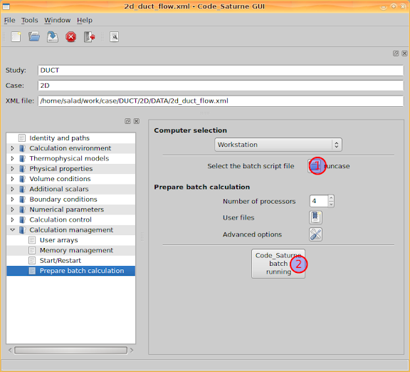
Then select the 'Number of processors', and click the button 'Code_Saturne batch running'. A console window will pop out and Code_Saturne will produce code to do the calculation. I assume that you are using more than one processor cores to calculate, and then you might be asked for your Linux system user password by openmpi before the calculation.
Leave the calculation console for minutes and then, if lucky enough, you will see the calculation finished normally. If so, the next step is to see the results and do post-processing.
Post-processing with ParaView
Please read Part III of this article.


Great job!
ReplyDeleteFor the density expression you can also use the formula editor when libmei is installed.
Thanks a lot :)
ReplyDeleteI know MEI, although I haven't tried it yet. Since the RC version is recently released, I am going to try it and publish new posts about it.
Thank you for the post. Does the modified fortran subroutine first need to be compiled? If so, which version of fortran needs to be used? Thanks. Sergio Perez.
ReplyDeleteHi Sergio,
ReplyDeleteYes, the fortran subroutines will be compiled before running the calculation. In my posts I suggested gfortran, which was also used by the compilation of Code_Saturne if you followed my posts to install that. Thereby you don't need to install an additional fortran compiler.
I guess g95 could work as well. Or you have Intel Fortran, which provides ifort.
Best regards,
Hi salad,
ReplyDeleteI'm trying to simulate the air flow around an airfoil profile. For this, I'm using Salome 5.1.3 & CS-2.0.0rc1. I've managed to obtain some pressure and velocity fields. Now, I want to obtain a plot of the pressure coefficients on the airfoil, but I don't know how to do this in Salome/CS. Any ideas?
Thanks, Marius
Hello Marius,
ReplyDeleteDid you use SALOME to plot the pressure and velocity fields? I suppose it shouldn't be difficult to plot pressure coefficients in ParaView, as there is a calculator filter there. With the help of the calculator you can based on the known parameters compute new parameter values which interests you.
Probably you could have a try :)
Best regards,
Hi,
ReplyDeleteIs there any tutorial in conjugate heat transfer like heatsink seating on top of an IC that is with varied amount of cooling air running arround?
email: code.saturne@yahoo.com
Thanks.
Hi Florante,
ReplyDeleteI don't have one on hand. However, although the geometry will be more complicated than a single flow duct, the calculation with Code_Saturne would be quite similar. That also depends on, in your case, if you have to consider turbulence models.
If the geometry is built up from duplicated units, python scripts in SALOME would be helpful very much.
Are you simulating a heat sink for an IC? It is interesting.
Best regards,
Hi Salad,
ReplyDeleteYes, I'm working on cooling an IC with heat sink. One factor for this type of work is determining the minimum amount of air to let it stay cool, then you can decide the fan size.
It would really be great if there will be some examples on how to set up this type of examples.
Thanks
Hi Florante,
ReplyDeleteUnfortunately I don't have an example like this at the moment. However, if in the process you study it, I would try to help fix the problems you encounter.
Good luck :)
Best regards,
Hi Salad,
ReplyDeleteI'm learning to tame this software right now. BTW, what's suppose to be the unit of the heat flux in the wall?
thanks
Florante
Hi Florante,
ReplyDeleteW/m2
Hi Salad...
ReplyDeleteRight now i'm learning using code saturne, and i use vers 1.3.3, and mesh generator GMSH.
I make a simple geometry, and try to run a laminar flow to the geometry, but it ended in error, and i can't figure what cause it.
Can i ask you in private (such as by email), and send you the mesh and xml file, so you can check where the problem is??
thank you
-Qohhar-
Hi Qohhar,
ReplyDeleteMy gmail account name is salad00. You can send the files to me and I'll try to help.
Otherwise, I will be quite busy next week and I am afraid I would only find some free time to help after I come back from Paris on 31 Aug.
Best regards,
Thanks for the quick reply and response.
ReplyDeleteI'll send you the files ASAP, and again, thanks for our help.
-Qohhar-
Hi Thank you for this tutorial.
ReplyDeleteI've just started using Code_Saturne 2.0-rc1 and I tried to run the stratified Junction tutorial which is written for Code-Saturne v1.3.3. I followed you instructions of this tutorial in cases where differences existed between the two versions. An the end though when I try to solve, I get this error:
chmod: cannot access `.../CASE1/SCRIPTS/runcase': No such file or directory
Do you have any idea why this might be?
My next plan was to do a channel flow example so thanks again for this tutorial.
Many Thanks,
Hi,
ReplyDeleteFollowing my previous question, I also tried running your example and got this error:
nohup: ignoring input and redirecting stderr to stdout
nohup: cannot run command `/Documents': Text file busy
Any idea what I'm doing wrong here?
Do we just choose the runcase file at the final step? When satrune asks you to save the file before running does one just save the file as a .xml file in the DATA directory?
Many Thanks
My problem is solved. ;)
ReplyDeleteHi Mina,
ReplyDeleteI am pretty glad that you have solved the problem by yourself. I was travelling so wasn't able to answer your questions.
Best wishes,
iḿ having the same problem, please how did you solve it?
ReplyDeletebasically i get this error message no my command console
ReplyDeletecp: target `saturne/ORIF/3D/SCRIPTS/runcase~' is not a directory
chmod: cannot access `saturne/ORIF/3D/SCRIPTS/runcase': No such file or directory
and im unable to execute the calculation
i tried to change the permissions to the runcase file but no change
possibly i must do it through chmod
can you please give me a hand with this issue.
Hello,
ReplyDeleteThank you for your perfect tutorial.
I'm going to write a fortran code to solve this problem by myself. Please can you help me deriving the main equations and bc's ?
I think the equations are:
- Heat equation
- Navier stocks equation (negligible momentum terms vs. viscosity terms)
Thanks